Intro + visualization

Quant Camp

Juan Tellez

UC Davis

September 14, 2026

Why are we here?

Why are we here?

  • Modern social science is increasingly methodologically sophisticated

  • A good (empirical) social scientist today needs to know:

    • statistics, probability, regression
    • (some) game theory
    • programming
    • managing AI agents
  • Picking up all of this stuff (at once, from a starting point of \(\approx\) 0) is challenging

Why are we here?

We’ve created quant camp to smooth this transition

Our goals:

  1. Learn some key data science concepts

  2. Get hands-on experience with quantitative data

  3. Develop a good, scientific workflow

Something changed

Most of you have used an LLM (ChatGPT, Claude, Gemini)

An LLM is a model that predicts text, trained on most of the written internet

  • you type, it writes back
  • it has read more R code than any human alive
  • it is often right, sometimes wrong, and always confident

From chatbot to agent

An agent is an LLM with tools and a loop

%%{init: {'theme': 'base', 'themeVariables': {'fontSize': '26px', 'primaryColor': '#e8eef6', 'primaryBorderColor': '#355B85', 'primaryTextColor': '#1a1a1a', 'lineColor': '#355B85'}}}%%
flowchart LR
  A[You describe<br>the goal] --> B[Agent reads<br>your files]
  B --> C[Agent writes<br>code]
  C --> D[Agent runs it]
  D --> E{Did it<br>work?}
  E -- no --> C
  E -- yes --> F[Agent reports<br>back to you]

It can read your files, write code, run it, read the error, and try again, until it thinks it’s done

What this means for you

This is how researchers now actually work: the agent writes much of the code

We need to:

  1. Read the code it writes
  2. Check that it did what you asked (this is harder than it sounds)
  3. Direct it: ask for the right thing, in the right way

Warning

The agent can see your files. It cannot see your intentions. If you don’t know what you want, neither does it.

Plan for today

  • Your first script, and your first agent
  • Reading what the agent wrote
  • How to plot data
  • Four key graphs, to show and to look

Your first script

Open the project

  1. Download rproject_camp.zip and extract it somewhere sensible (not Downloads)

  2. Open the folder and double-click rproject_camp.Rproj. RStudio opens with the project loaded

  3. In the Files pane (bottom right), open code/plot-un-votes.R

Everything we do this week happens inside this folder:

  • code/ for scripts
  • data/ for data
  • figures/ for plots

Run it, top to bottom

Run the whole script (Cmd/Ctrl + Shift + Enter, or click Source)

The first time, it will install a couple of packages. Wait for it to finish.

When it’s done, look in the figures/ folder. There should be a file called figure.pdf. Open it.

That’s a script: a text file of R commands that runs from top to bottom and produces something. Nothing is done by hand.

Starting the agent

Claude Code only sees the folder it was started in. So, every time:

  1. Open a terminal (Terminal on Mac, PowerShell on Windows). Not the one inside RStudio

  2. Go to your project folder: type cd and a space, then drag the folder from Finder / File Explorer into the terminal, and hit enter

    cd ~/Desktop/rproject_camp
  3. Check: ls should list code, data, figures

  4. Type claude

Ask it “what folder am I in?” If the answer isn’t your project, it’s in the wrong place.

Note

Prefer an app? The Claude Code desktop app does the same thing: open it, pick the project folder, start typing.

🚨 Your turn: make it yours 🚨

Change three things in plot-un-votes.R, running the script after each one:

  1. Pick different countries. Find where the two countries are chosen and swap in two (or three) of your own. Country names have to match the data exactly

  2. Name the output. figure.pdf tells you nothing. Change the file name to something that describes what’s in it

  3. Make it prettier. With claude running in your project folder, ask it to improve the plot: a title, real axis labels, percentages on the y-axis, a nicer theme. Whatever you want. Then run the script again

What just happened?

  • What did the agent change? Can you find each change in the code?
  • Did it do anything you didn’t ask for?
  • Could you explain every line of the script now? Which ones can’t you?

The agent wrote it, but it’s your script. The rest of camp is about being able to say what every line does.

Reading what the agent wrote

What I asked for, and what I got

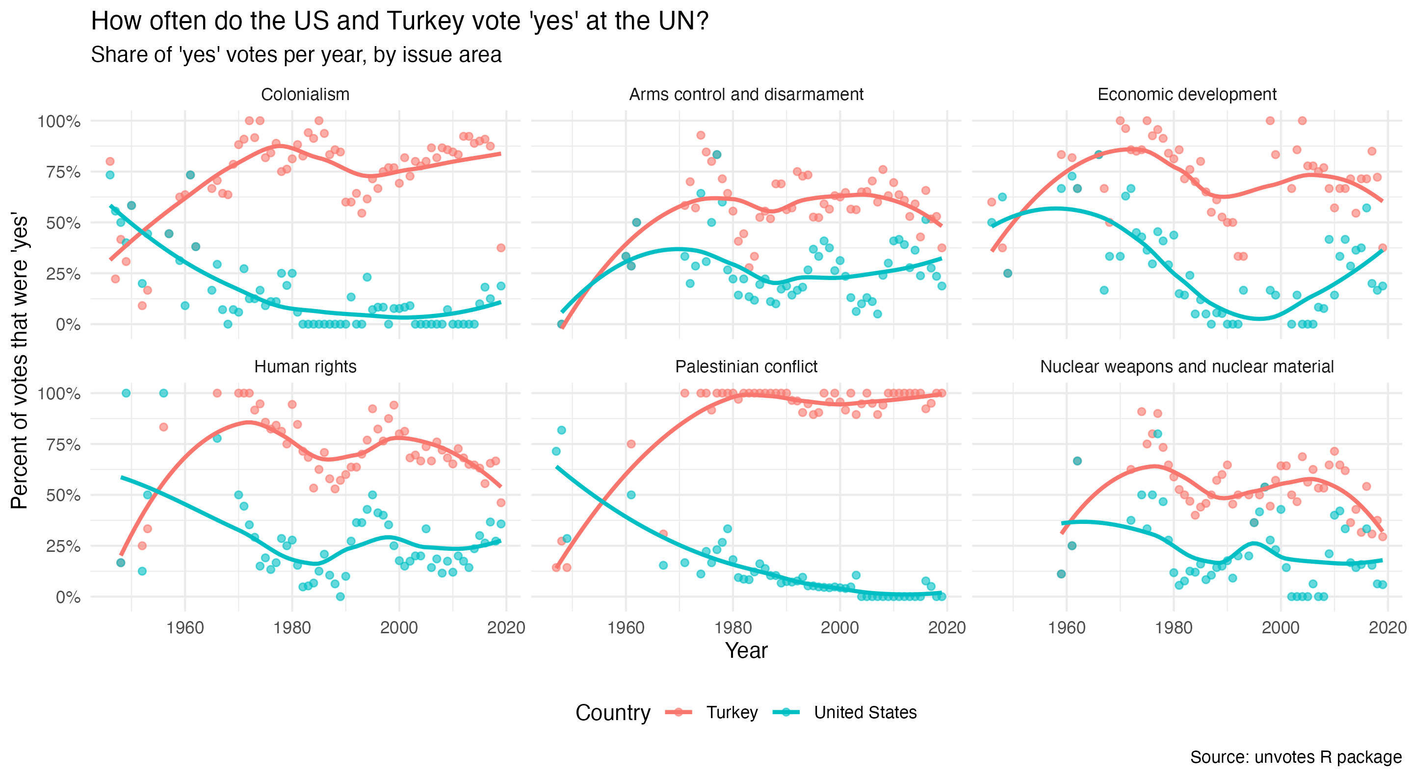
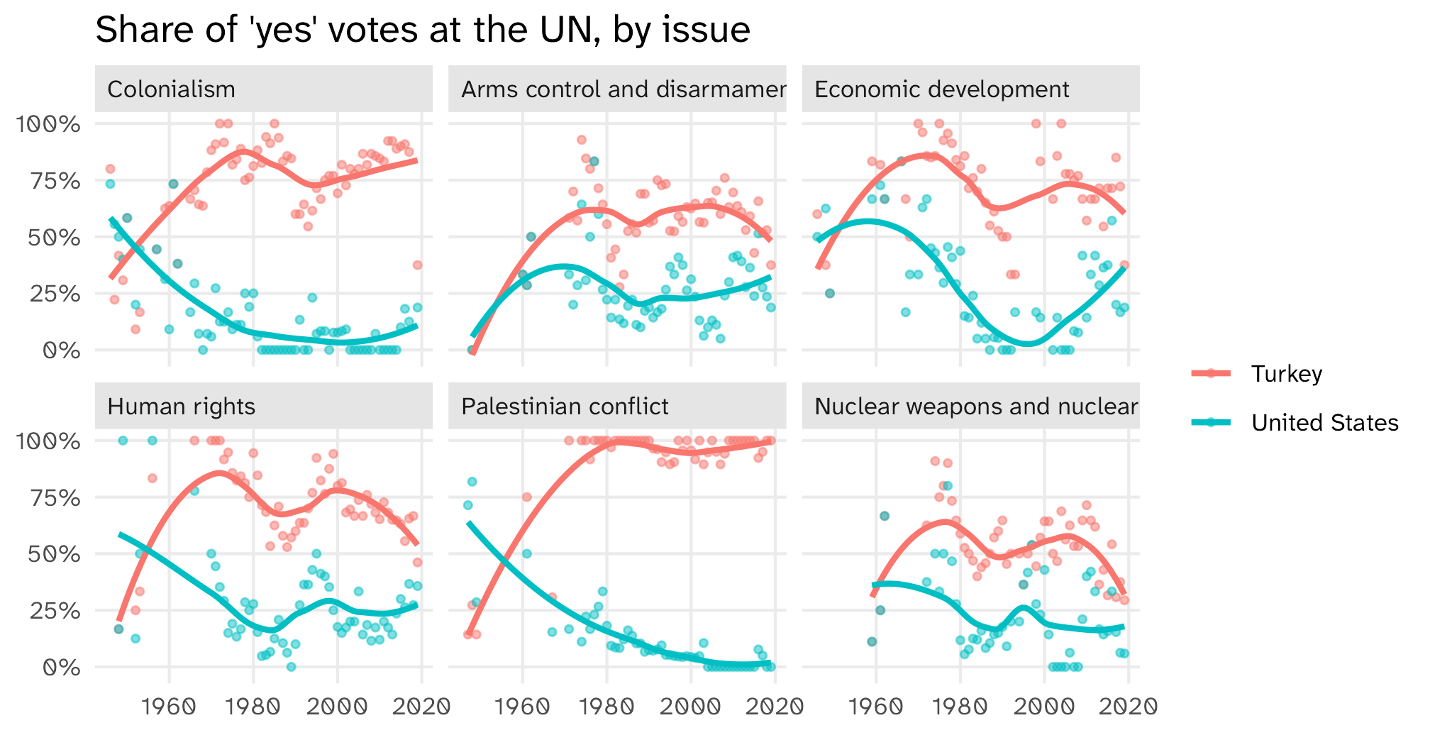
I asked: “Make the plot prettier: add a title, real axis labels, show the y-axis as percentages, and use a nicer theme.”

It changed only the plotting block. Here it is:

ggplot(un_yes, aes(x = year, y = percent_yes, color = country)) +
  geom_point(alpha = 0.6) +                    # lighter points so the trend line stands out
  geom_smooth(method = "loess", se = FALSE) +
  facet_wrap(~ issue) +
  # percent_yes is a proportion (0 to 1), so show the axis as 0% to 100%
  scale_y_continuous(labels = scales::percent) +
  # title and human-readable axis / legend labels
  labs(
    title = "How often do the US and Turkey vote 'yes' at the UN?",
    subtitle = "Share of 'yes' votes per year, by issue area",
    x = "Year",
    y = "Percent of votes that were 'yes'",
    color = "Country",
    caption = "Source: unvotes R package"
  ) +
  # clean theme with the legend along the bottom
  theme_minimal() +
  theme(legend.position = "bottom")

The plot it made

Did it do what you asked?

Look at line 7 again:

ggplot(un_yes, aes(x = year, y = percent_yes, color = country)) +
  geom_point(alpha = 0.6) +
  geom_smooth(method = "loess", se = FALSE) +
  facet_wrap(~ issue) +
  scale_y_continuous(labels = scales::percent) +
  labs(
    title = "How often do the US and Turkey vote 'yes' at the UN?",
    subtitle = "Share of 'yes' votes per year, by issue area",
    x = "Year",
    y = "Percent of votes that were 'yes'",
    color = "Country",
    caption = "Source: unvotes R package"
  ) +
  theme_minimal() +
  theme(legend.position = "bottom")

The title hard-codes the two countries. If you changed the countries in task 1, your title is now wrong, and nothing warned you.

The agent did exactly what you asked. It just didn’t know what you meant. Checking is your job.

This is a good workflow

Look at what you did

  • You worked inside a project folder, with code/, data/, and figures/
  • You ran a script from top to bottom. It loaded its own packages and produced a file
  • The file path was here("figures", "figure.pdf"), which works on any computer that has the folder
  • You changed one line (the countries) and re-ran the whole thing
  • Nothing was done by hand. No clicking, no copy-paste into Word

That is the whole idea of a reproducible workflow. You’ll do it every day this week.

Example: the “conference fix”

Say this UN plot goes in a paper. Months later, a reviewer says: drop Turkey, add Brazil and France. Change one line, re-run:

filter(country == "United States" | 
       country == "Turkey")
filter(country == "United States" | 
       country == "Brazil" | country == "France")
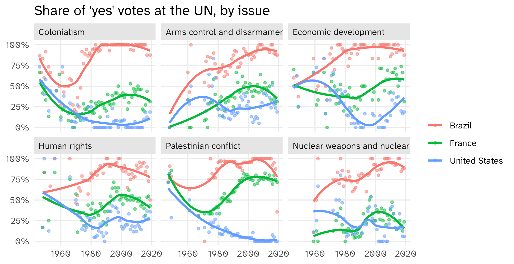
Everything downstream of that line (the figure, the file in figures/, the paper that reads it) updates on its own. Bad workflow: rebuild it by hand ❌ Good workflow: change one line, re-run ✅

File paths

File paths can be confusing if you’re not used to them

Two approaches to file paths, absolute and relative

Absolute paths:

ggsave(filename = "/Users/juan/Dropbox/RAs/econ-extort/figures/my_plot.pdf")

Downsides: long, tedious, and only works on your computer (not reproducible!)

Rprojects facilitate the use of clean, relative paths:

ggsave(filename = "figures/my_plot.pdf")

Short, works for anyone working from the same .Rproj as you

Working with .Rproj files is part of a good workflow

The rules are written down

Your project folder has a file called CLAUDE.md. The agent reads it every time it starts. Here is what it says:

# Instructions for AI coding agents

This is an R project for UC Davis Quant Camp. I am a beginner. Follow these rules.

## Where things go

- Scripts go in `code/`. Name them by day and task, e.g. `code/01_five_graphs.R`
- Raw data goes in `data/`. Never edit or overwrite files in `data/`.
- Cleaned data goes in `data/clean/`.
- Every plot is saved with `ggsave()` into `figures/`. Tell me the file name.

## How to write R here

- Use the tidyverse. Use `=` for assignment and the `|>` pipe.
- Use `here::here()` for every file path. Never write an absolute path.
- Every script must run top to bottom from a fresh R session (`library()` calls at the top).
- Comment the code so a beginner can follow what each block does.
- After you write code, run it and show me the output (rows, columns, or the plot).

## When unsure

- If you don't know what a column means, ask me before guessing.
- If a step drops or duplicates rows, say so explicitly.

A project an agent can work in is a project a collaborator can work in. Or you, in six months.

🚨 Your turn: tell it who you are 🚨

Open CLAUDE.md in RStudio (it’s in the Files pane) and add a section at the bottom:

## Who I am

- My name is ... and I study ...
- I have never used R before (or: I used R once, in ...)
- When you explain code, ...

Fill in the three lines however you like. Save the file.

Then quit Claude (/exit), start it again, and ask: “what do you know about me?”

How to plot data

The Gapminder dataset

The Gapminder dataset
country continent year lifeExp pop gdpPercap
Afghanistan Asia 1952 29 8425333 779
Afghanistan Asia 1957 30 9240934 821
Afghanistan Asia 1962 32 10267083 853
Afghanistan Asia 1967 34 11537966 836
Afghanistan Asia 1972 36 13079460 740
Afghanistan Asia 1977 38 14880372 786

Rows are observations

The Gapminder dataset
country continent year lifeExp pop gdpPercap
Afghanistan Asia 1952 29 8425333 779
Afghanistan Asia 1957 30 9240934 821
Afghanistan Asia 1962 32 10267083 853
Afghanistan Asia 1967 34 11537966 836
Afghanistan Asia 1972 36 13079460 740

In a dataset, rows are observations

The data we observe for Afghanistan in the year 1952

Rows are observations

Sample from the General Social Survey
id age degree race sex
1 47 Bachelor White Male
2 61 High School White Male
3 72 Bachelor White Male
4 43 High School White Female
5 55 Graduate White Female

In survey data, an observation is typically a person who took the survey (a respondent)

Columns are variables

The Gapminder dataset
country continent year lifeExp pop gdpPercap
Afghanistan Asia 1952 28.80 8425333 779.45
Afghanistan Asia 1957 30.33 9240934 820.85
Afghanistan Asia 1962 32.00 10267083 853.10
Afghanistan Asia 1967 34.02 11537966 836.20
Afghanistan Asia 1972 36.09 13079460 739.98

In a dataset, columns are variables

Life expectancy and GDP per capita are some of the variables in our data

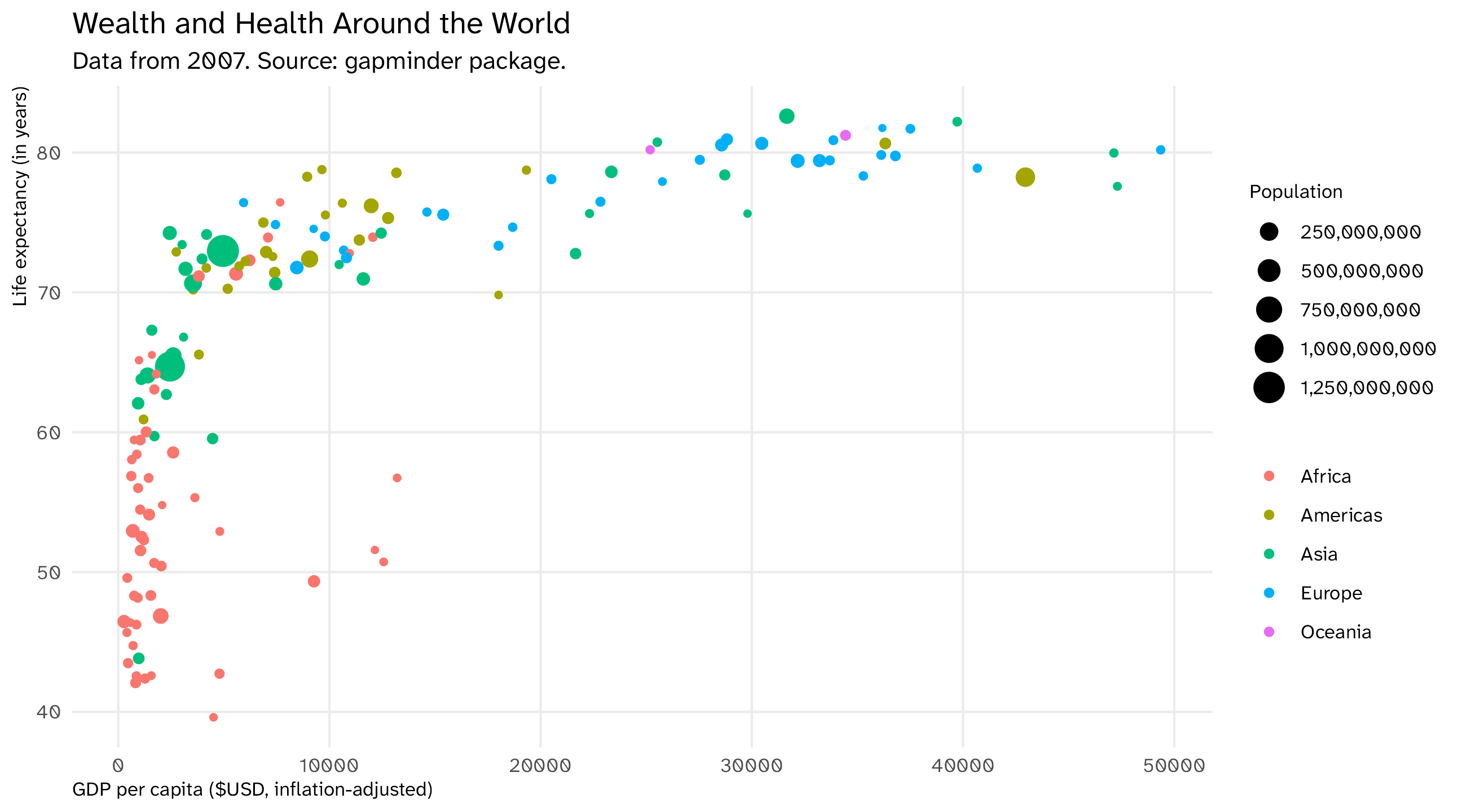
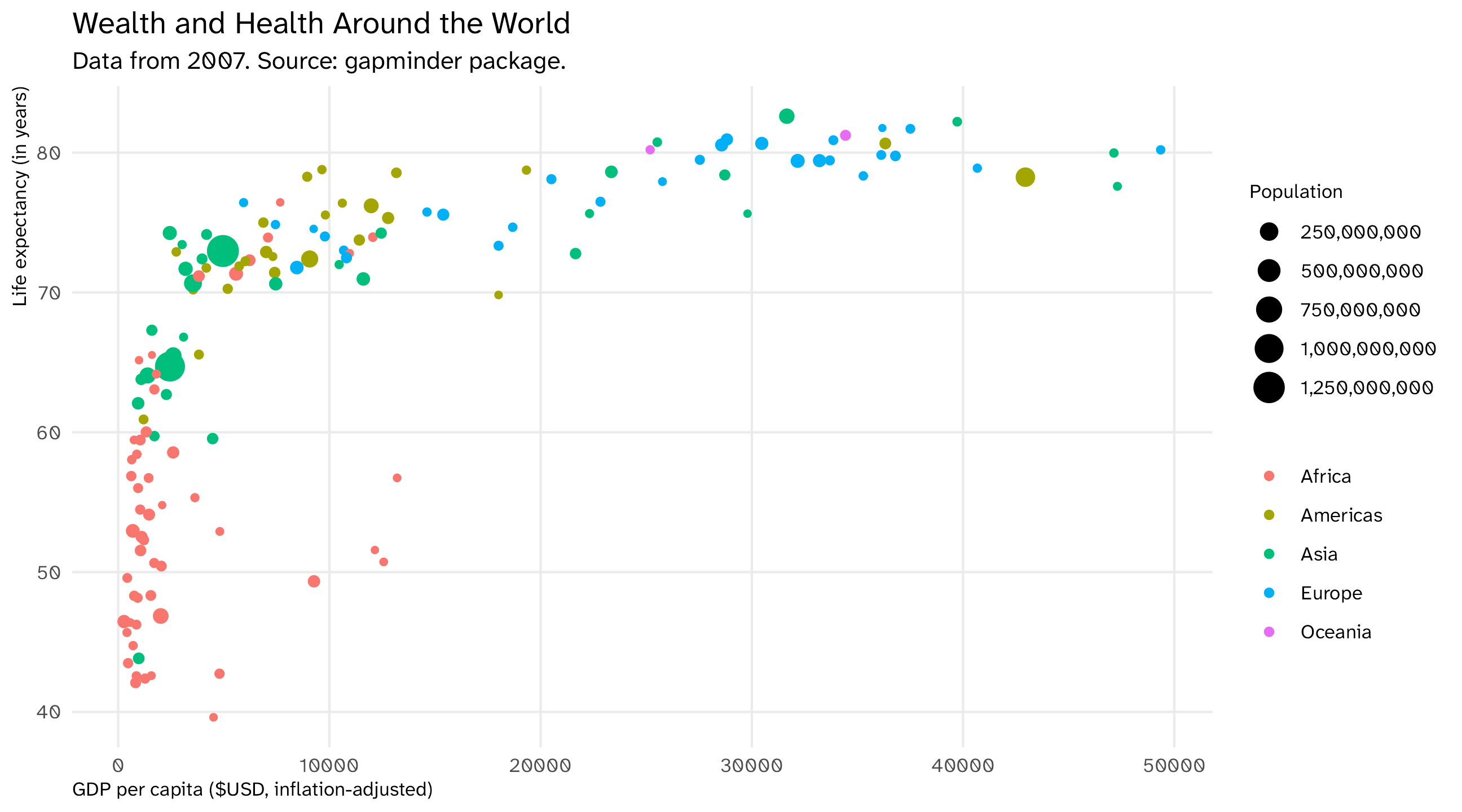
The final graph

Mapping data to aesthetics
The Gapminder dataset
country continent year lifeExp pop gdpPercap
Afghanistan Asia 1952 28.80 8425333 779.45
Afghanistan Asia 1957 30.33 9240934 820.85
Afghanistan Asia 1962 32.00 10267083 853.10
Afghanistan Asia 1967 34.02 11537966 836.20
Afghanistan Asia 1972 36.09 13079460 739.98

Aesthetics are the visual properties of the plot: x-axis, y-axis, color, size, shape, etc.

Geometries are the visual elements that represent the data: points, lines, bars, etc.

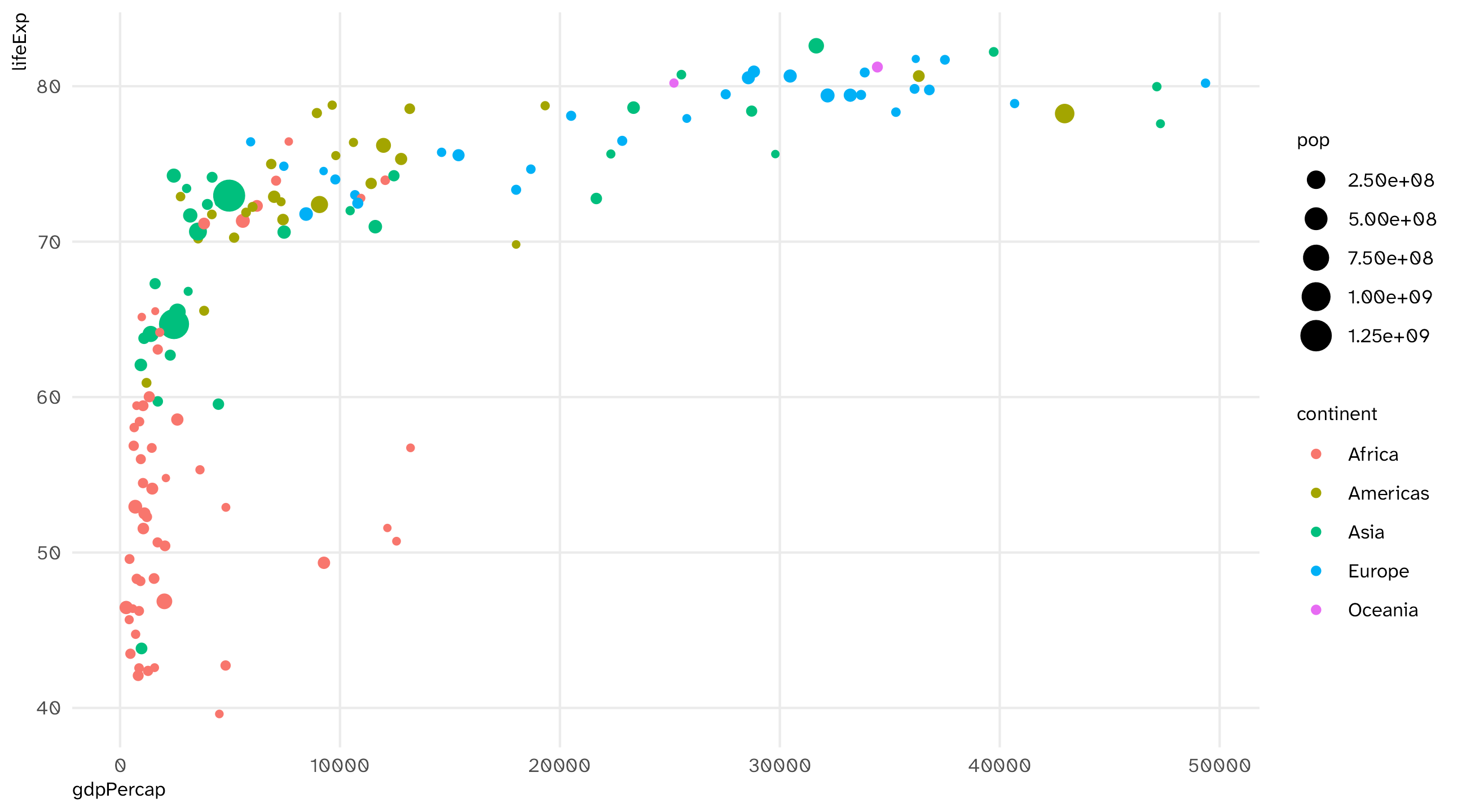
How has gapminder been mapped onto the aesthetics of this plot? And with what geometries?

Mapping data to aesthetics

Data Aesthetic Geometry
GDP per capita x-axis Point
Life expectancy y-axis Point
Continent Color Point
Population Size Point
  1. Take the data,

  2. map it onto an aesthetic,

  3. and visualize it with a geometry

In R

Subset of Gapminder dataset (year = 2007)
country continent year lifeExp pop gdpPercap
Afghanistan Asia 2007 43.8 31889923 974.6
Albania Europe 2007 76.4 3600523 5937.0
Algeria Africa 2007 72.3 33333216 6223.4
Angola Africa 2007 42.7 12420476 4797.2
Argentina Americas 2007 75.3 40301927 12779.4
Australia Oceania 2007 81.2 20434176 34435.4
Mapping data to aesthetics
Data aes() geom_
gdpPercap x geom_point()
lifeExp y geom_point()
continent color geom_point()
pop size geom_point()

Use the variable names exactly as they appear in the data, map them onto the exact function names in R

ggplot(): our first function

ggplot()

ggplot: specify the data

ggplot(data = gap_07)

Use aes() (short for aesthetic) to map variables to aesthetics
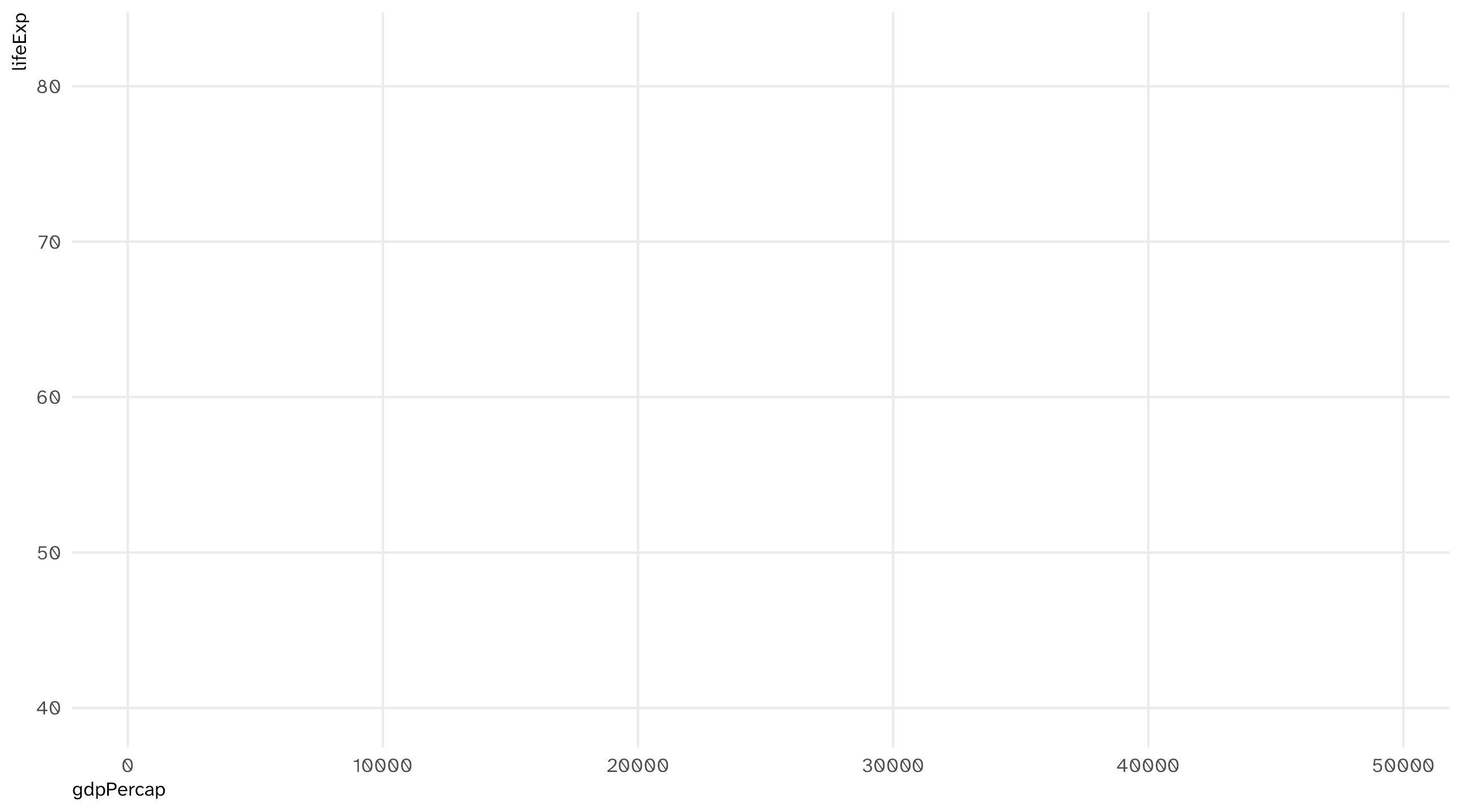
ggplot(data = gap_07, aes(x = gdpPercap, y = lifeExp))

add geometries and layers using +

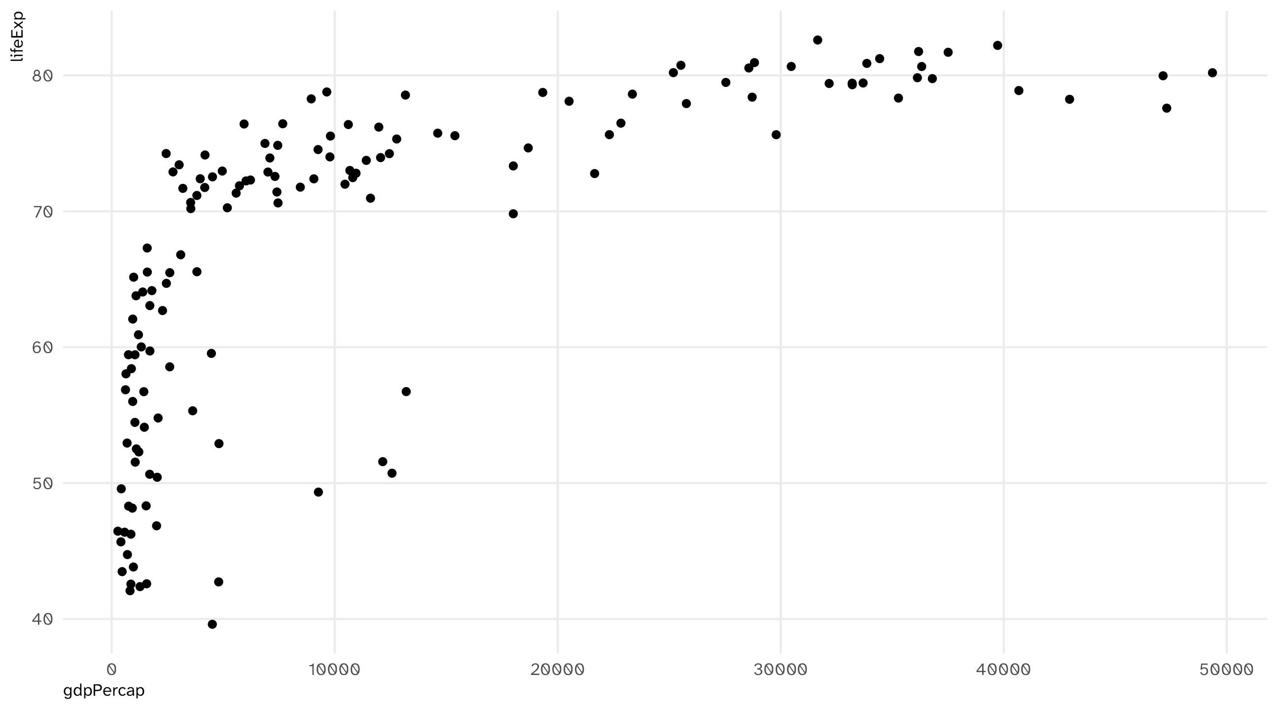
ggplot(data = gap_07, aes(x = gdpPercap, y = lifeExp)) + geom_point()

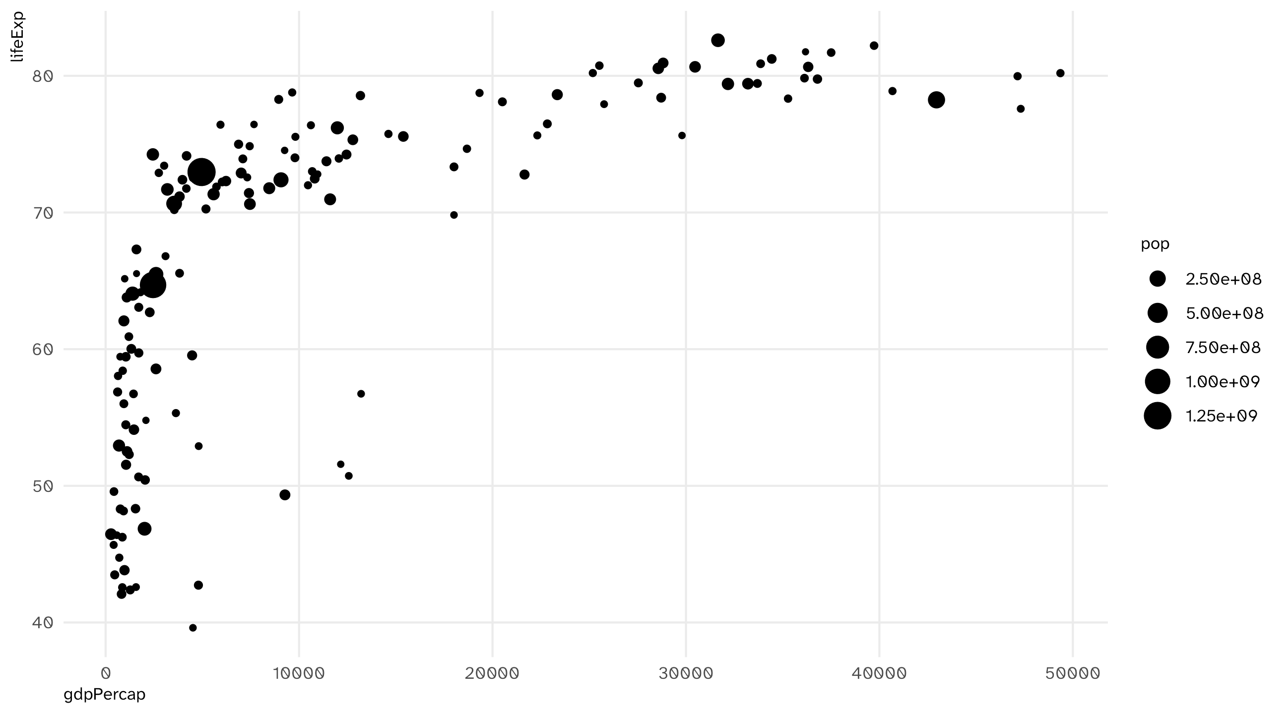
mapping population to size in aes()

ggplot(data = gap_07, aes(x = gdpPercap, y = lifeExp, size = pop)) + 
  geom_point()

mapping continent to color in aes()
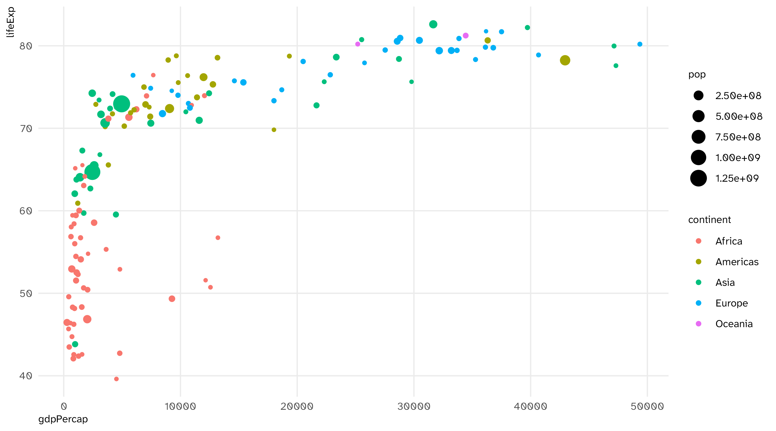
ggplot(data = gap_07, aes(x = gdpPercap, y = lifeExp, size = pop, color = continent)) + 
  geom_point()

Other layers: add the missing titles with labs()
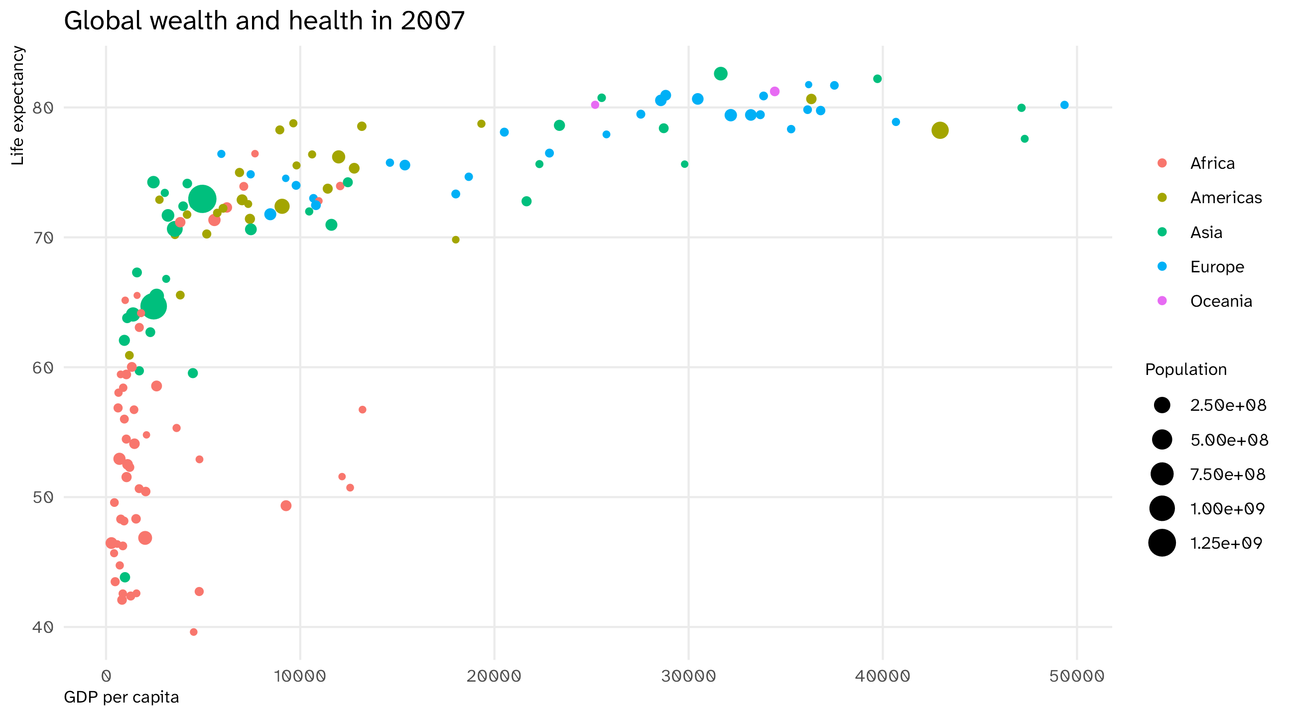
ggplot(data = gap_07, aes(x = gdpPercap, y = lifeExp, size = pop, color = continent)) + 
  geom_point() + 
  labs(x = "GDP per capita", y = "Life expectancy",  title = "Global wealth and health in 2007", size = "Population", color = NULL)

Notice we are adding layers to the plot with +

The final formula

  1. Take the data,
ggplot(data = gap_07)
  1. map it onto aesthetics,
ggplot(data = gap_07, aes(x = gdpPercap, y = lifeExp, size = pop, color = continent))
  1. add geometries and other layers
ggplot(data = gap_07, aes(x = gdpPercap, y = lifeExp, size = pop, color = continent)) + 
  geom_point() + labs(x = "GDP per capita", y = "Life expectancy", title = "Global wealth and health in 2007", size = "Population", color = NULL)

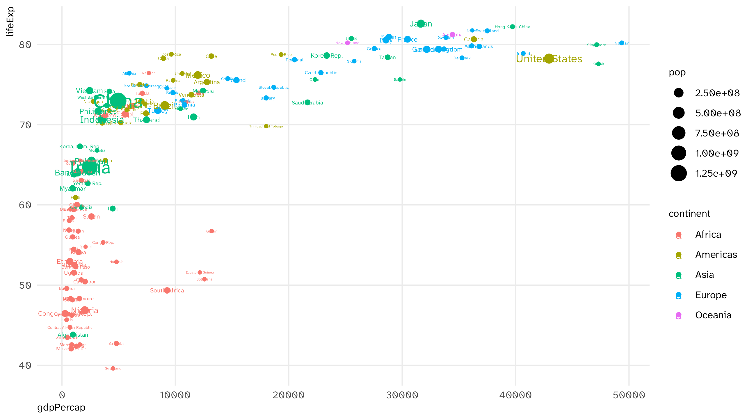
What’s that country way out on the bottom right?
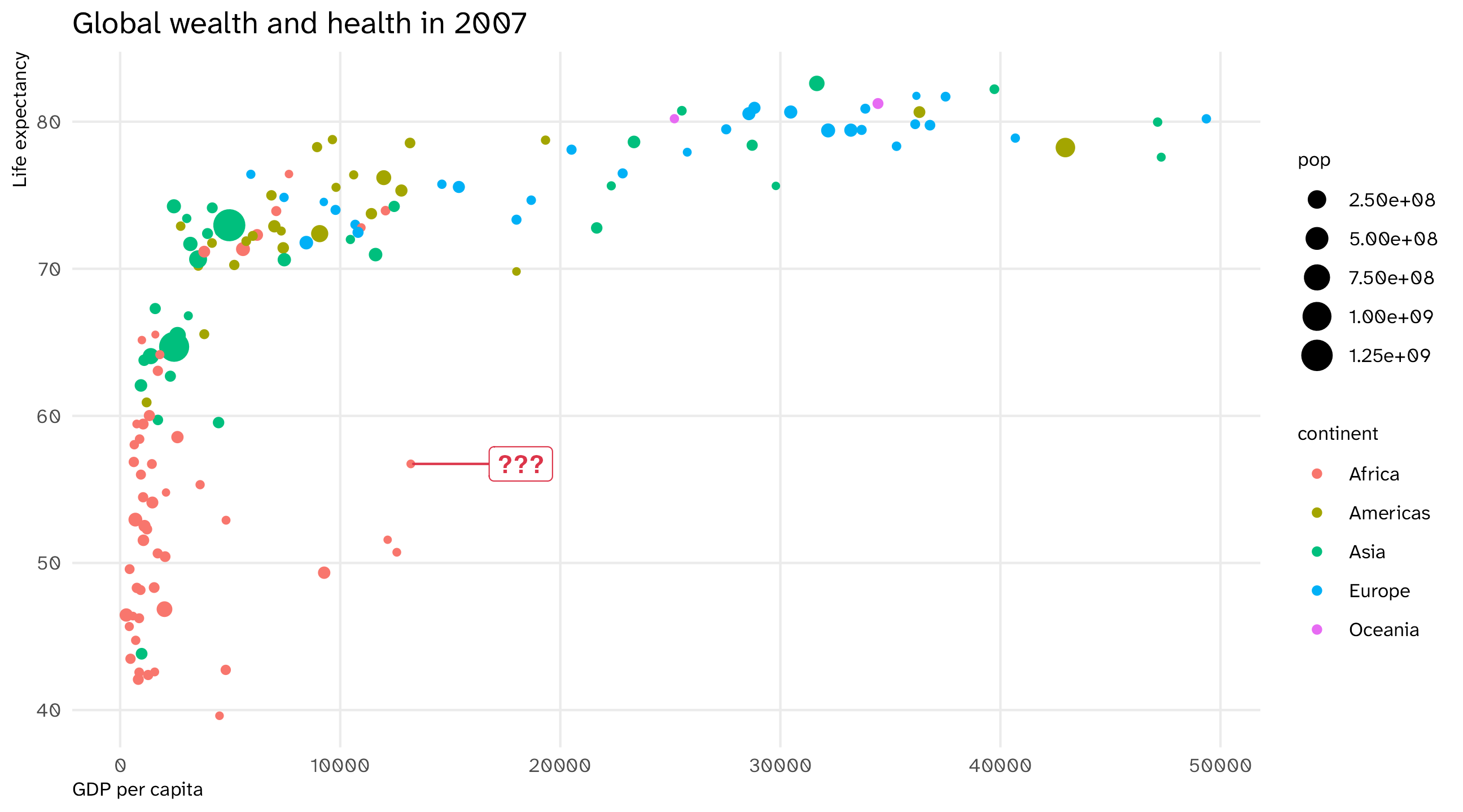
🚨 Your turn: try labelling the points 🚨

  1. Add labels to each point by mapping country names onto the label aesthetic within aes()

  2. Add geom_text layer to your plot to plot the names

  3. Once you do this, use Claude to change the plot so only that country’s is highlighted

Map country names to label aesthetic

ggplot(data = gap_07, aes(x = gdpPercap, y = lifeExp, size = pop, color = continent, label = country)) + geom_point()

Plot the labels

ggplot(data = gap_07, aes(x = gdpPercap, y = lifeExp, size = pop, color = continent, label = country)) + geom_point() + geom_text() 

What did we do?

Data Aesthetic Geometry
gdpPercap x geom_point()
lifeExp y geom_point()
continent color geom_point()
pop size geom_point()
country label geom_text()

Take your data, map it onto an aesthetic, represent with a geometry

Using graphs to show and to look

Two jobs for a graph

  1. To show. Convey an idea/argument
    • In a paper, talk, tweet
  2. To look. You don’t know what’s in the data, the graph helps you find out
    • Is the variable shaped the way I think? Are there impossible values? Did something change halfway through?

Key questions

  • What am I trying to show?

    • (a distribution, a relationship, a comparison, an amount)
  • What kind of variables do I have?

    • (continuous, discrete, something in between)
  • What aesthetics and geometries do I need for this plot?

    • (x-axis, y-axis, color, size, shape, etc.)

What kind of variable do I have?

General Social Survey
id age degree race num_kids
1 47 Bachelor White 3
2 61 High School White 0
3 72 Bachelor White 2
4 43 High School White 4
5 55 Graduate White 2

Continuous variables take on lots of values (GDP, population, income, age, etc.)

What kind of variable do I have?

General Social Survey
id age degree race num_kids
1 47 Bachelor White 3
2 61 High School White 0
3 72 Bachelor White 2
4 43 High School White 4
5 55 Graduate White 2

Discrete or categorical variables takes on a few values, often “qualitative” (yes/no, 1/0, race, etc.)

Visualize a relationship: the scatterplot (#1)

The Gapminder dataset
country continent year lifeExp pop gdpPercap
Afghanistan Asia 1952 28.80 8425333 779.45
Afghanistan Asia 1957 30.33 9240934 820.85
Afghanistan Asia 1962 32.00 10267083 853.10
Afghanistan Asia 1967 34.02 11537966 836.20
Afghanistan Asia 1972 36.09 13079460 739.98
Afghanistan Asia 1977 38.44 14880372 786.11

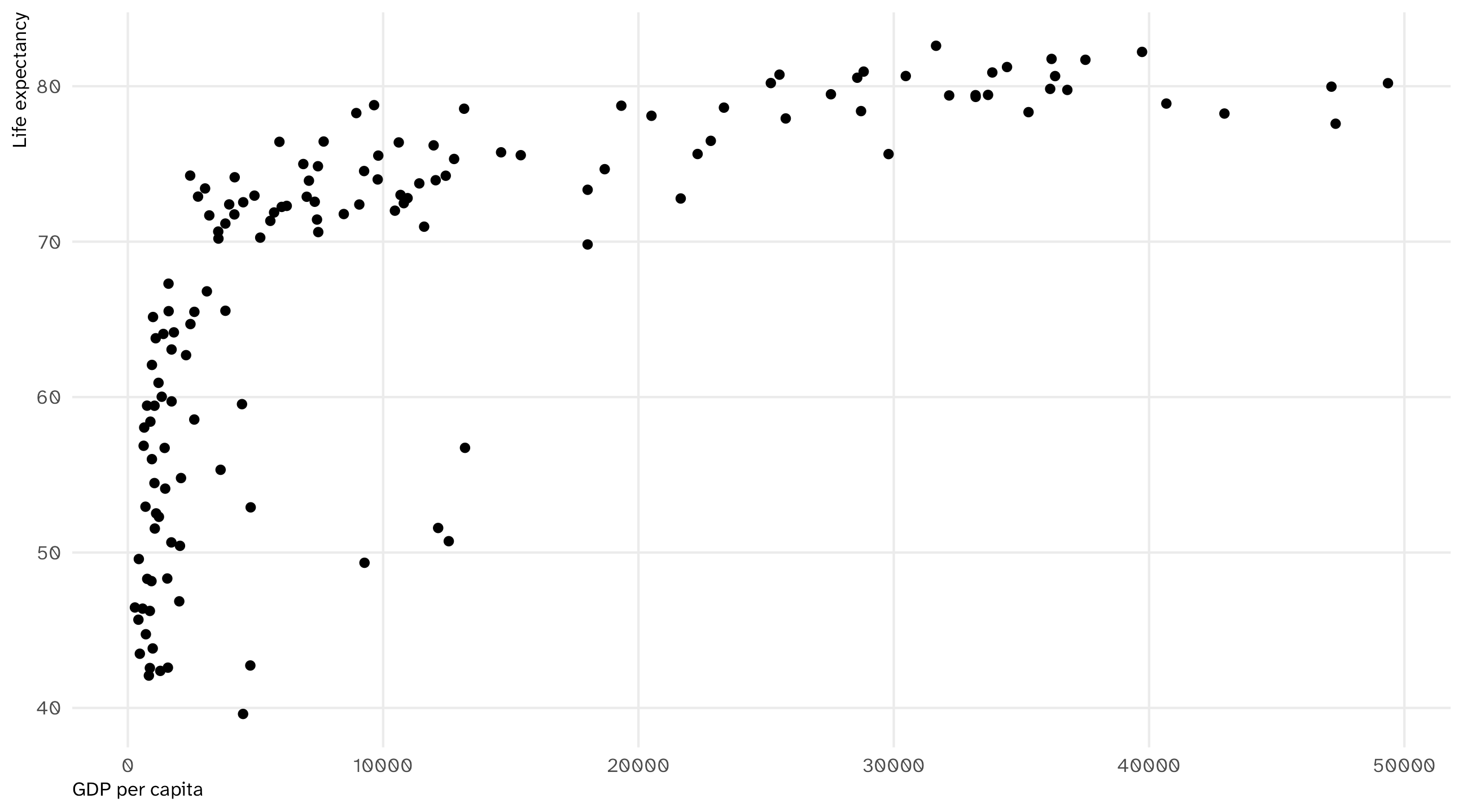
What is the relationship between GDP per capita and life expectancy around the world? How quickly does life expectancy increase as GDP increases?

The scatterplot

Every Gapminder country-year, GDP per capita against life expectancy:
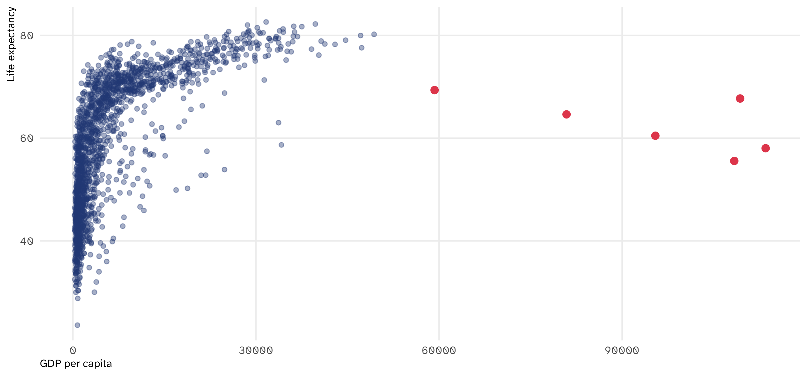
Code
ggplot(gapminder, aes(x = gdpPercap, y = lifeExp)) + 
  geom_point(alpha = .4, color = blue) + 
  geom_point(data = filter(gapminder, gdpPercap > 50000), color = red, size = 2.5) + 
  labs(x = "GDP per capita", y = "Life expectancy")

The red points are Kuwait, 1952 to 1972. Error, or real? (Real: oil and a tiny population.) You don’t know until you check

The grammar of scatterplots

Gapminder, every country-year
country year gdpPercap lifeExp
Afghanistan 1952 779 29
Afghanistan 1957 821 30
Afghanistan 1962 853 32
Afghanistan 1967 836 34
Afghanistan 1972 740 36
Afghanistan 1977 786 38
Mapping the data
Data Aesthetic Geometry
gdpPercap x geom_point()
lifeExp y geom_point()

What we put on the X and Y axis matters: convention is to put the theorized cause on the X axis and effect on the Y axis

Scatterplots in R

Code
ggplot(gap_07, aes(x = gdpPercap, y = lifeExp)) + geom_point(size = 1.5) + 
  labs(x = "GDP per capita",
       y = "Life expectancy")

Basic scatterplot uses the x-axis, y-axis, and a point geometry

The time series
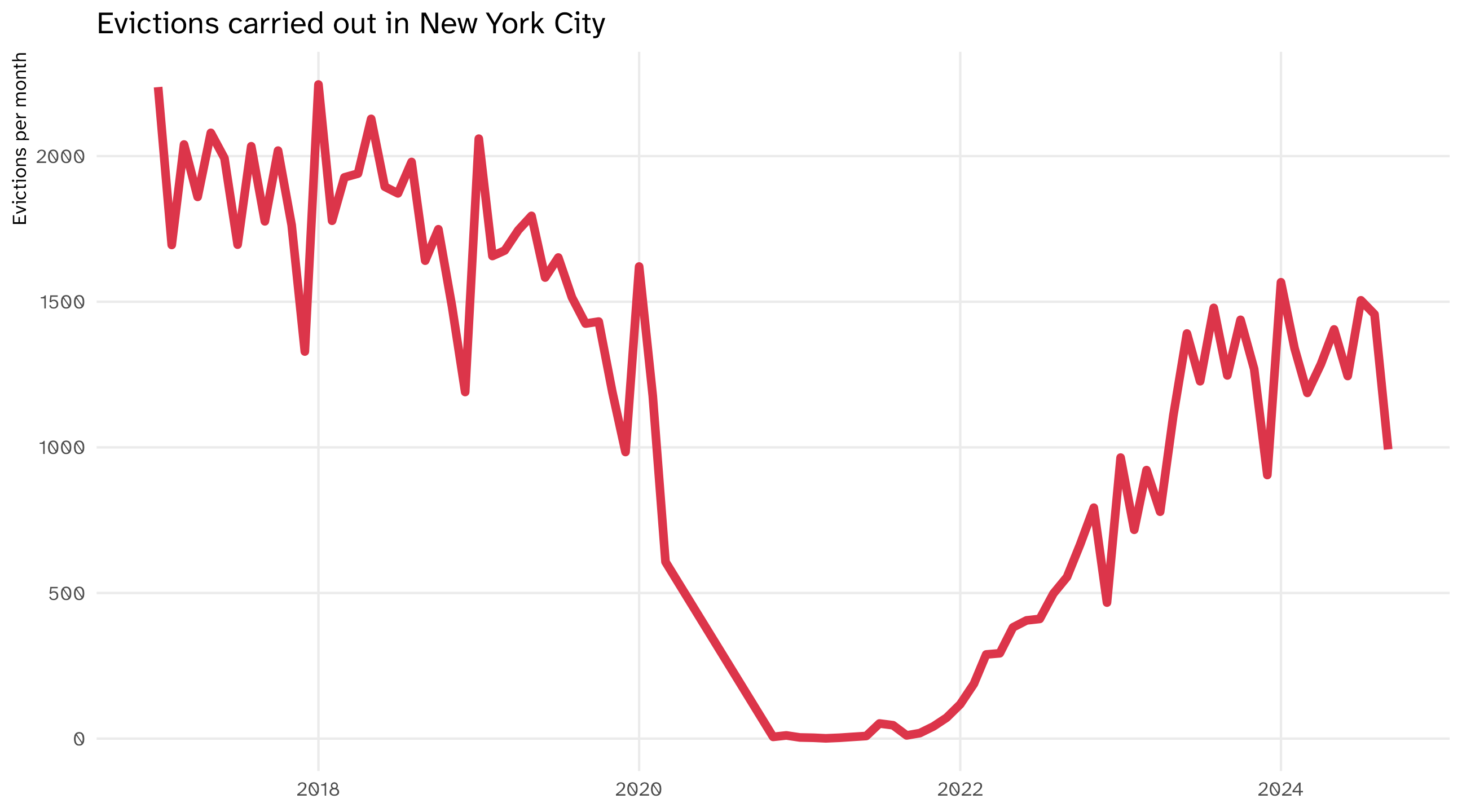
The time series uses a line to show you how a variable (y-axis) moves over time (x-axis)

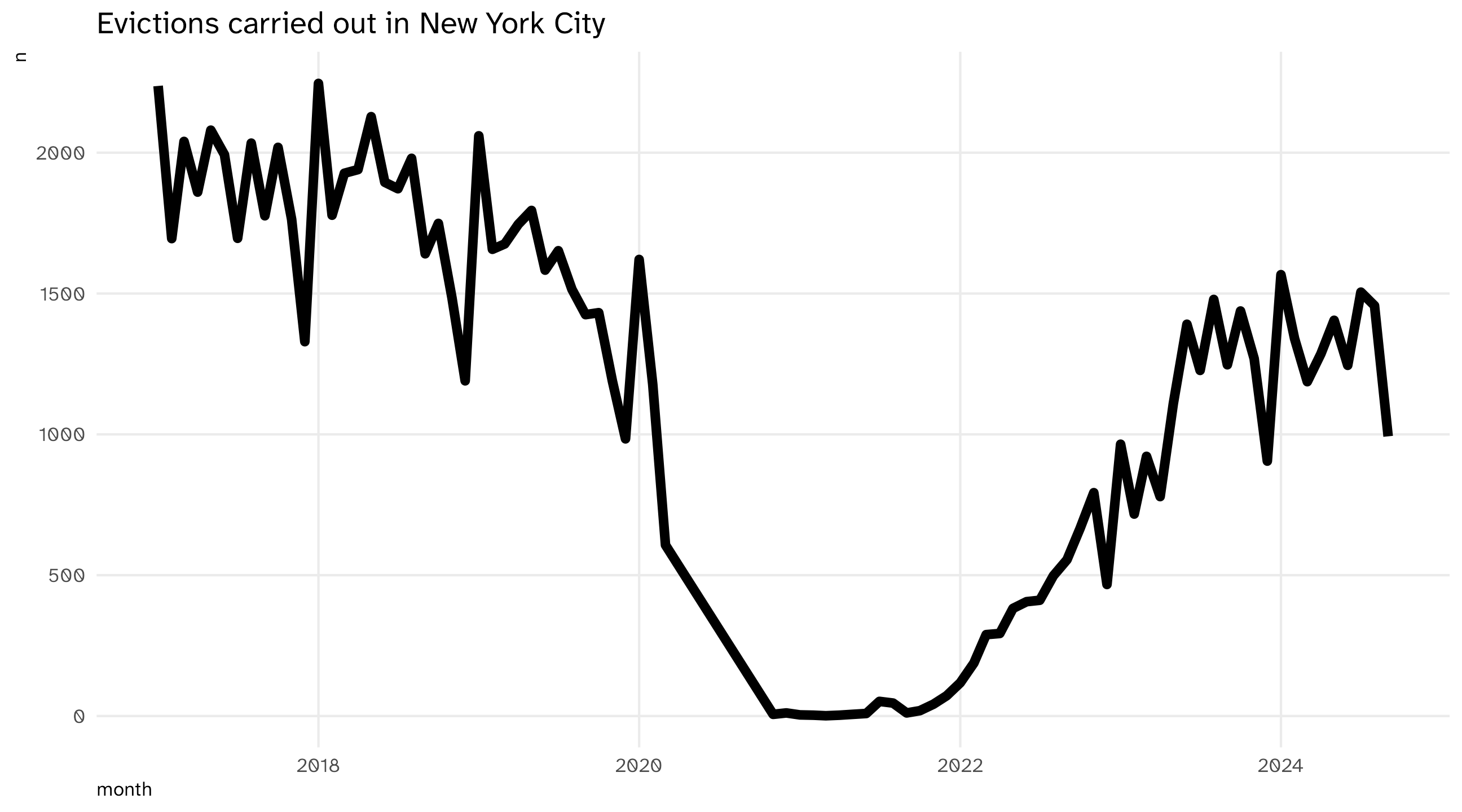
A cliff. Real, or did the data stop?
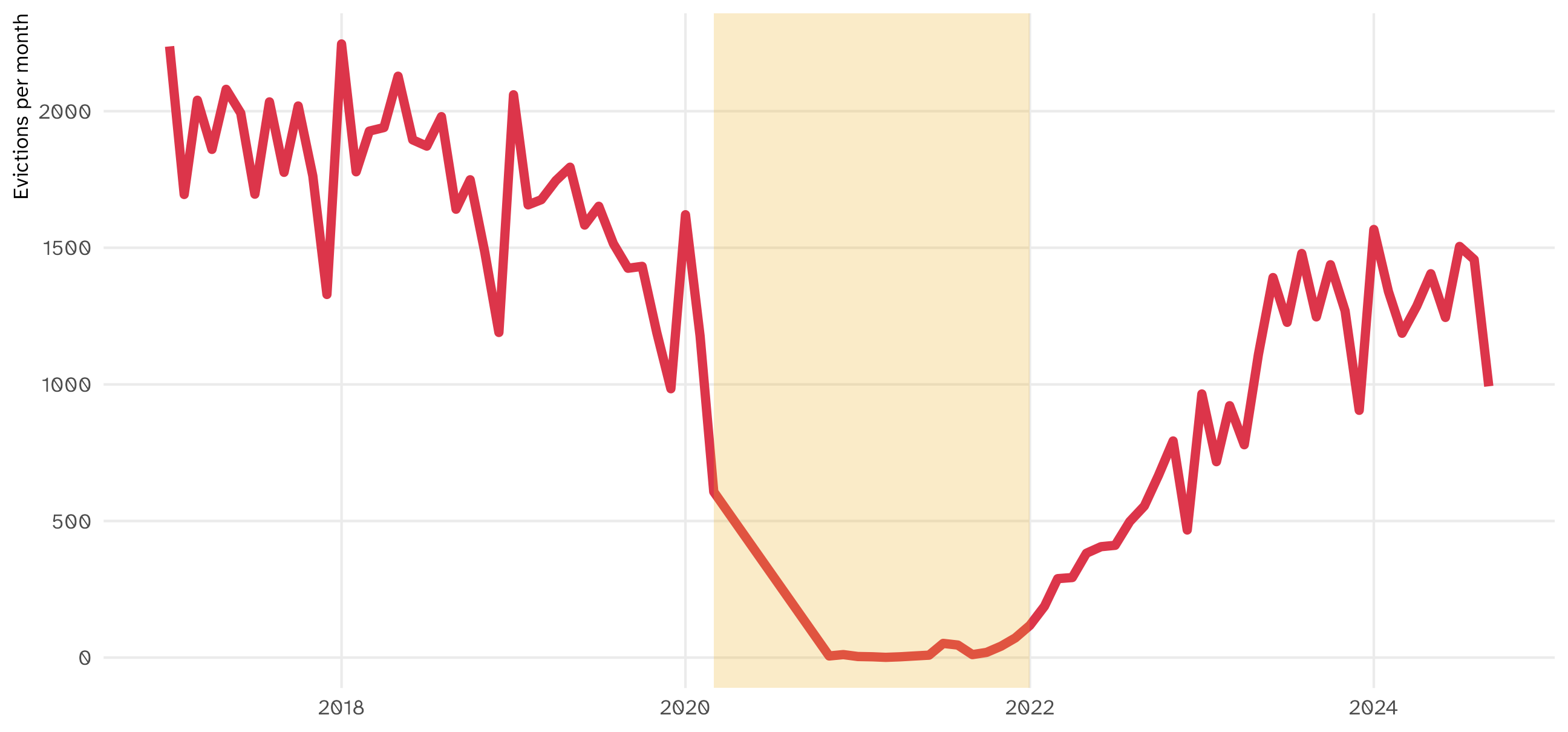
Evictions drop to almost zero in early 2020. The world changed (a COVID eviction moratorium), or the data changed (collection stopped, a source switched)? The plot can’t tell you

It tells you to go find out, before you compute a “2020 average” or a “trend”

The grammar of time series

Evictions, counted by month
month n
2017-01-01 2237
2017-02-01 1695
2017-03-01 2040
2017-04-01 1860
2017-05-01 2080
2017-06-01 1993
Mapping the data
Data Aesthetic Geometry
month x geom_line()
n y geom_line()


Notice the new geometry, geom_line(). One row per month, one point per row, and the line connects them in order

The time series

Code
ggplot(evict_month, aes(x = month, y = n)) + geom_line(linewidth = 2) + labs(title = "Evictions carried out in New York City")

Note

You can change line width using the linewidth argument

🚨 Your turn: 💸Recession💸 🚨

  • Type and run economics to see the data

  • Type and run ?economics to read about the data

  • Make a time series of unemployment (which variable?) over time

  • Can you identify the recessions?

  • Have your agent plot the other variable side-by-side with your current plot. Look at what it added to your code

multiple time series

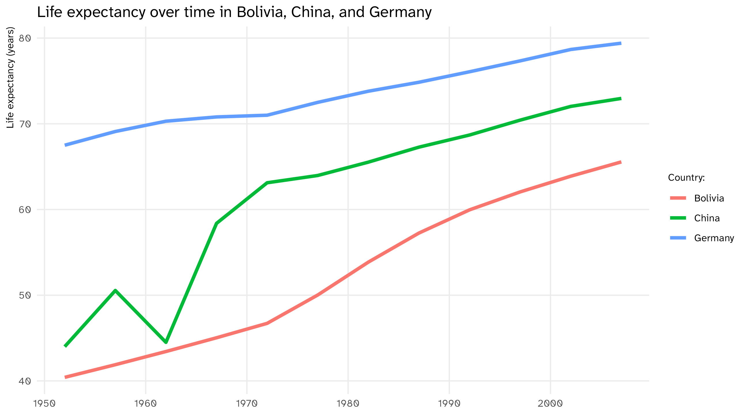
Multiple time series allow us to compare trends across units

Start from scratch

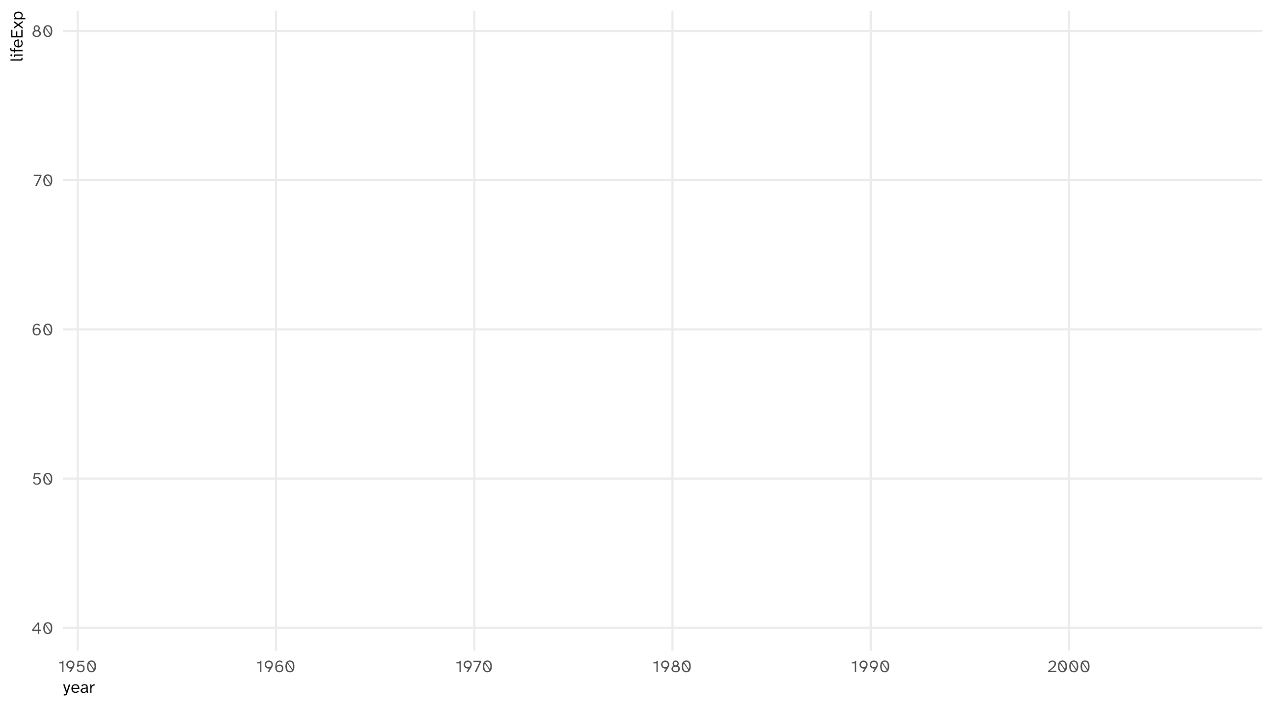
ggplot(data = gapminder_sample) 

Add aesthetics

ggplot(data = gapminder_sample, aes(x = year, y = lifeExp)) 

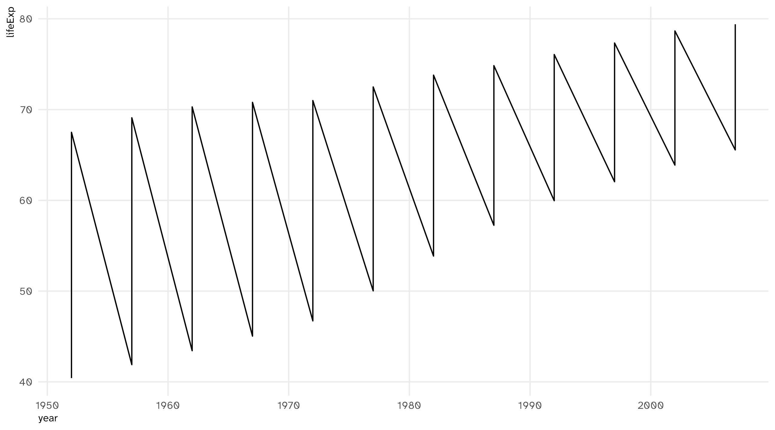
Add geometry: 🤢

ggplot(data = gapminder_sample, aes(x = year, y = lifeExp)) + geom_line()

Problem: R doesn’t “know” there should be separate lines, makes one instead

Why one line?

geom_line() does one thing: connect the points, in order of x

We told R what goes on x (year) and y (lifeExp). We did not tell it which rows belong together

What R sees
country year lifeExp
Bolivia 1952 40.41
China 1952 44.00
Germany 1952 67.50
Bolivia 1957 41.89
China 1957 50.55
Germany 1957 69.10

So for 1952 it has three points, one per country, and it connects all of them before moving on to 1957

The zigzag is Bolivia → China → Germany → Bolivia → …

Tell R which rows belong together

The rows that belong together share a country. Map that variable onto an aesthetic, and R can tell them apart
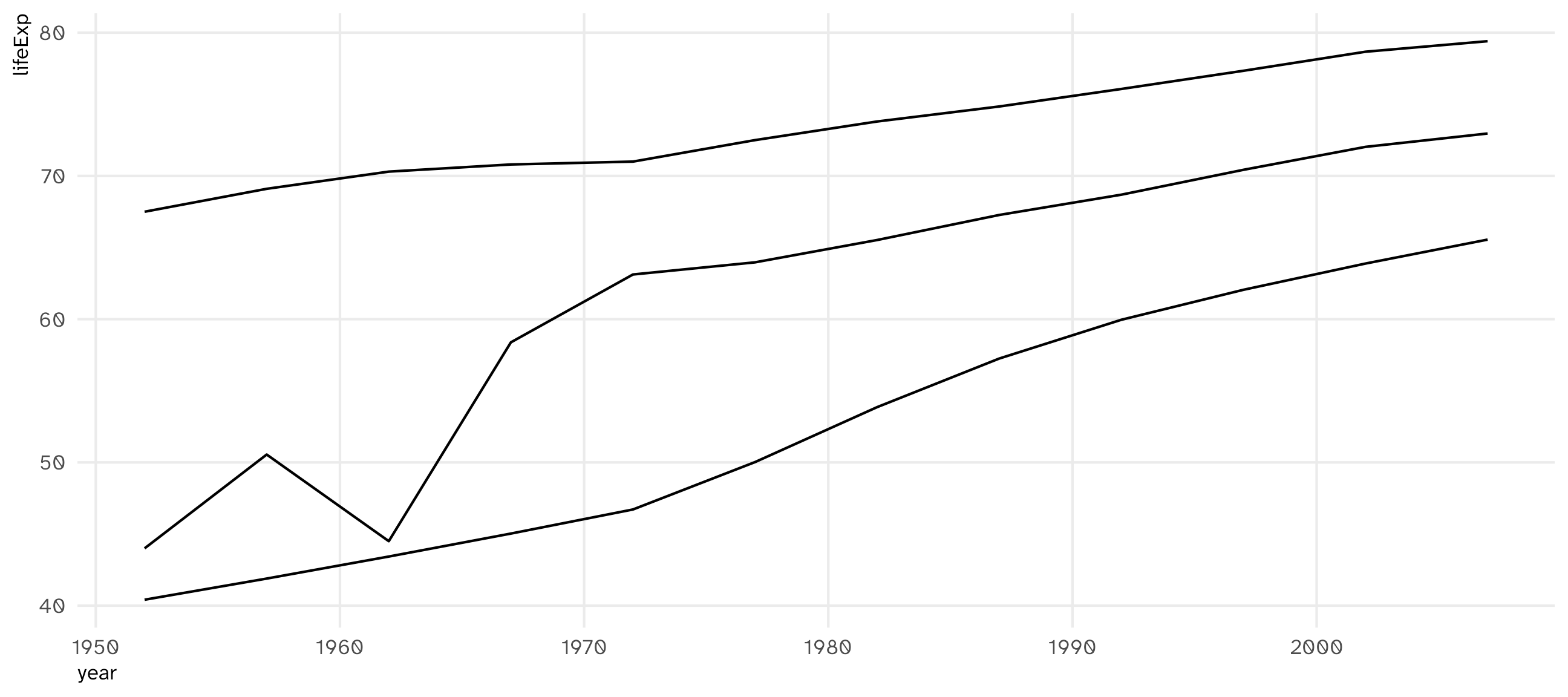
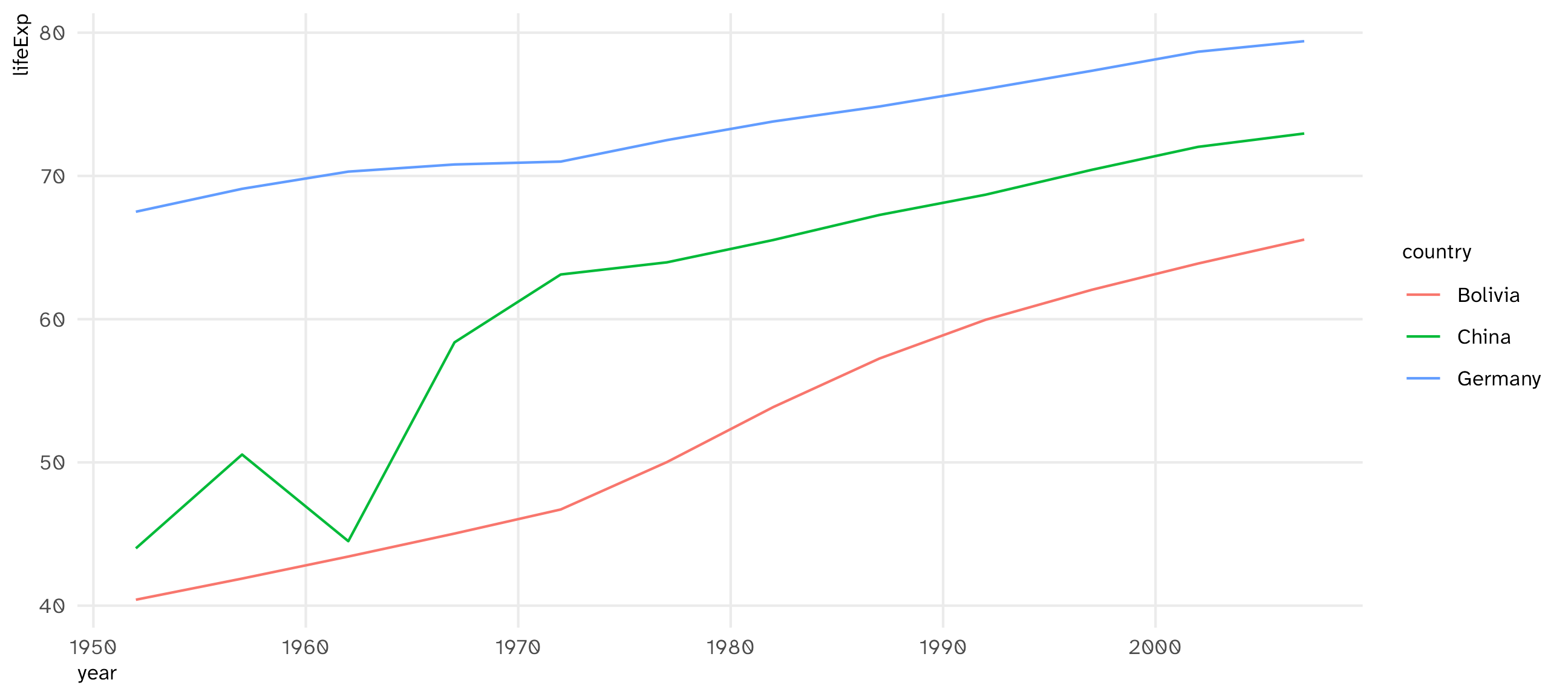
ggplot(data = gapminder_sample, 
       aes(x = year, y = lifeExp, group = country)) + 
  geom_line()

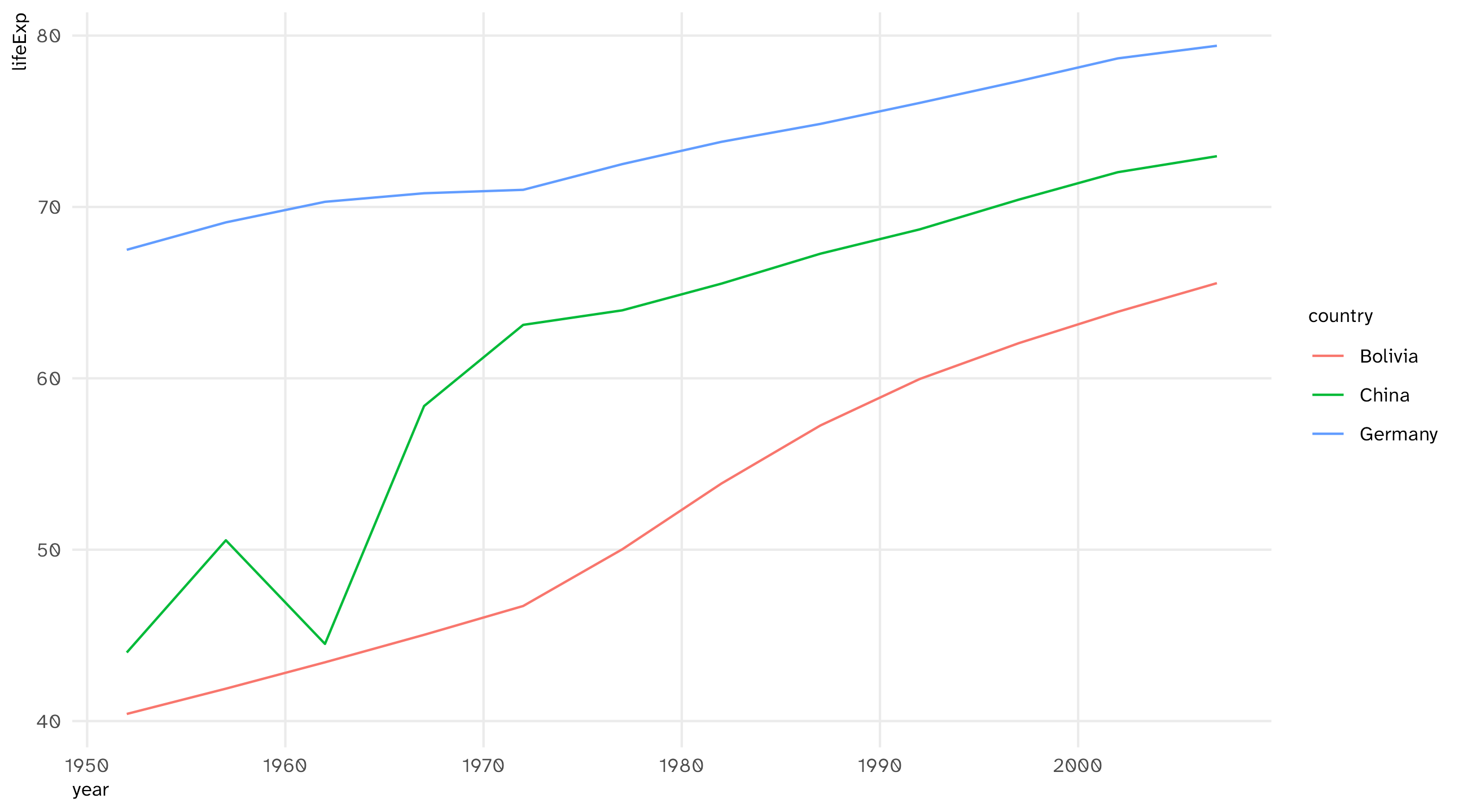
group: separate lines, but which is which?

ggplot(data = gapminder_sample, 
       aes(x = year, y = lifeExp, color = country)) + 
  geom_line()

color: separate lines and a legend

using color to separate lines

ggplot(data = gapminder_sample, aes(x = year, y = lifeExp, color = country)) + geom_line()

Same recipe as always: time on x, the variable on y, and the unit (country, state, person) on color

Visualize distributions: the histogram (#3)

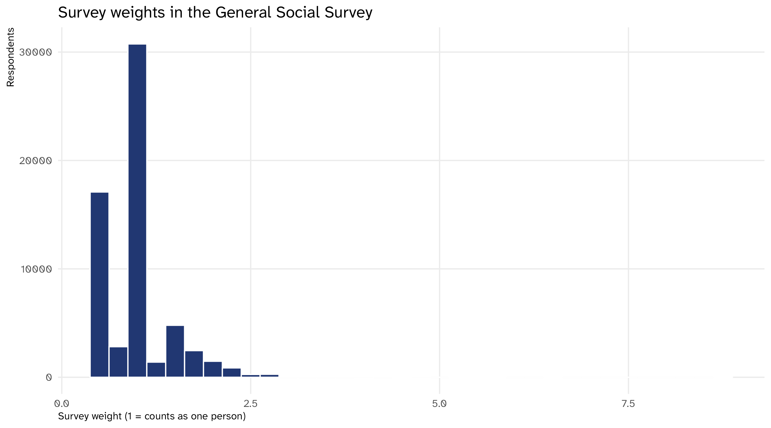
Surveys come with weights: how many people in the population each respondent “stands for.” A weight of 2 means that person counts double

General Social Survey, 1972 to 2016
year age sex marital wtssall
1972 23 Female Never Married 0.44
1972 70 Male Married 0.89
1972 48 Female Married 0.89
1972 27 Female Married 0.89
1972 61 Female Married 0.89
Average weight
avg_weight
1

The average weight is 1 (by construction). How informative is that number? Is there a “typical” weight?

The histogram

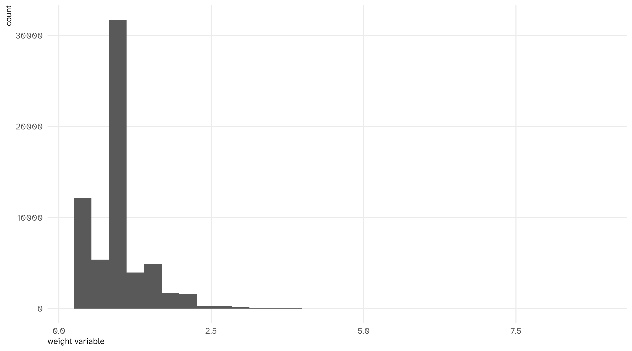
A histogram shows you how a continuous variable is distributed

It shows you how many observations (respondents) fall into different “bins” of values (weights)

Why does the axis go to 9?
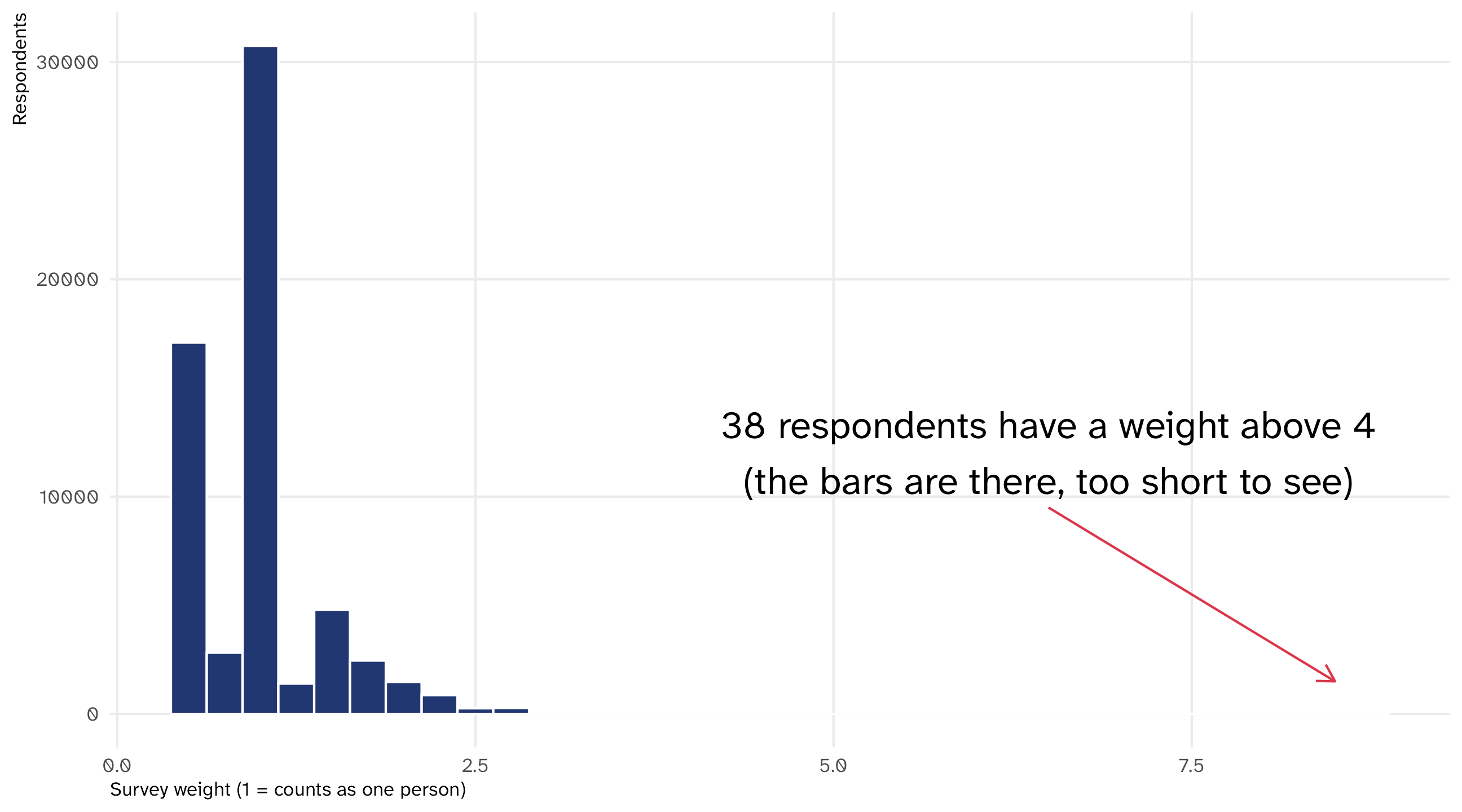
Most respondents count as about one person. A few count as eight

Why do these respondents have so much weight?

The heaviest respondents
year age sex marital wtssall
2012 51 Male Married 8.74
2004 20 Male Never Married 6.43
2008 81 Female Married 6.41
2006 41 Female Widowed 5.73
2006 23 Male Never Married 5.73
2006 27 Male Never Married 5.73
2004 57 Female Married 5.51
  • The GSS interviews one adult per household. Someone from a household with four adults stands for more people than someone who lives alone
  • From 2004 on, the GSS stopped chasing every hard-to-reach household. It followed up with a random half of them, and gave those interviews double weight
  • Almost all of the tail is 2004 to 2012

The histogram helped us understand our data better

The grammar of histograms

General Social Survey
year age sex wtssall
1972 23 Female 0.44
1972 70 Male 0.89
1972 48 Female 0.89
1972 27 Female 0.89
1972 61 Female 0.89
Mapping the data
Data Aesthetic Geometry
wtssall x geom_histogram()


Notice the new geometry, geom_histogram(); and that a histogram only uses the x-axis! R counts the rows in each bin for you

The histogram

Code
ggplot(weights, aes(x = wtssall)) + 
  geom_histogram()

Note

The default is 30 bins. binwidth = .25 (or bins = 50) changes how fine the picture is; try a few

🚨 Your turn: organs 🫁🧠 🚨

  • Grab the organdata dataset (from the socviz package)

  • Make a histogram of countries’ organ donation rate (donors)

  • Then make a grouped histogram, where groups are defined by whether donors have to opt in or opt out of donating (opt)

  • Now ask the agent to mark the country with the highest donation rate on the plot. Which country is it? Look at what it added to your code

Compare quantities: the barplot (#4)

Afrobarometer, Ethiopia (2020)
age region urban protest
27 Amhara urban No, would never
66 Amhara rural No, would never
25 Oromia rural No, would never
19 Amhara urban Yes, once or twice
25 Oromia rural No, would never
42 Amhara rural No, would never
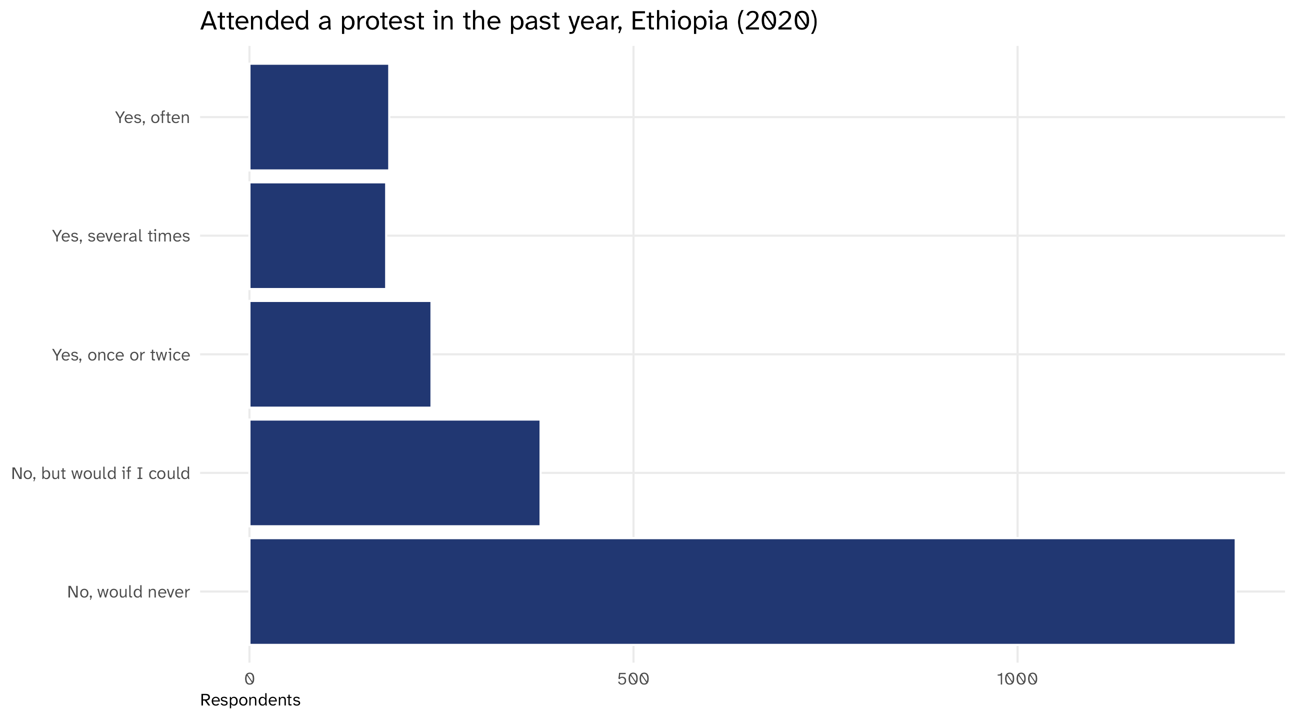
Attended a protest in the past year
protest n
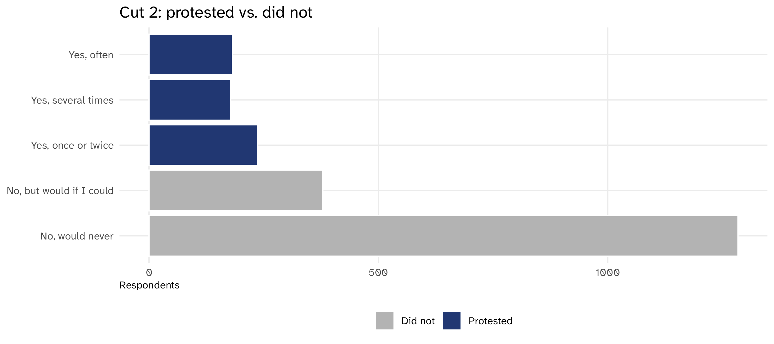
No, would never 1284
No, but would if I could 379
Yes, once or twice 237
Yes, several times 178
Yes, often 182

Survey question: in the past year, have you attended a demonstration or protest march? How many people gave each answer?

The barplot

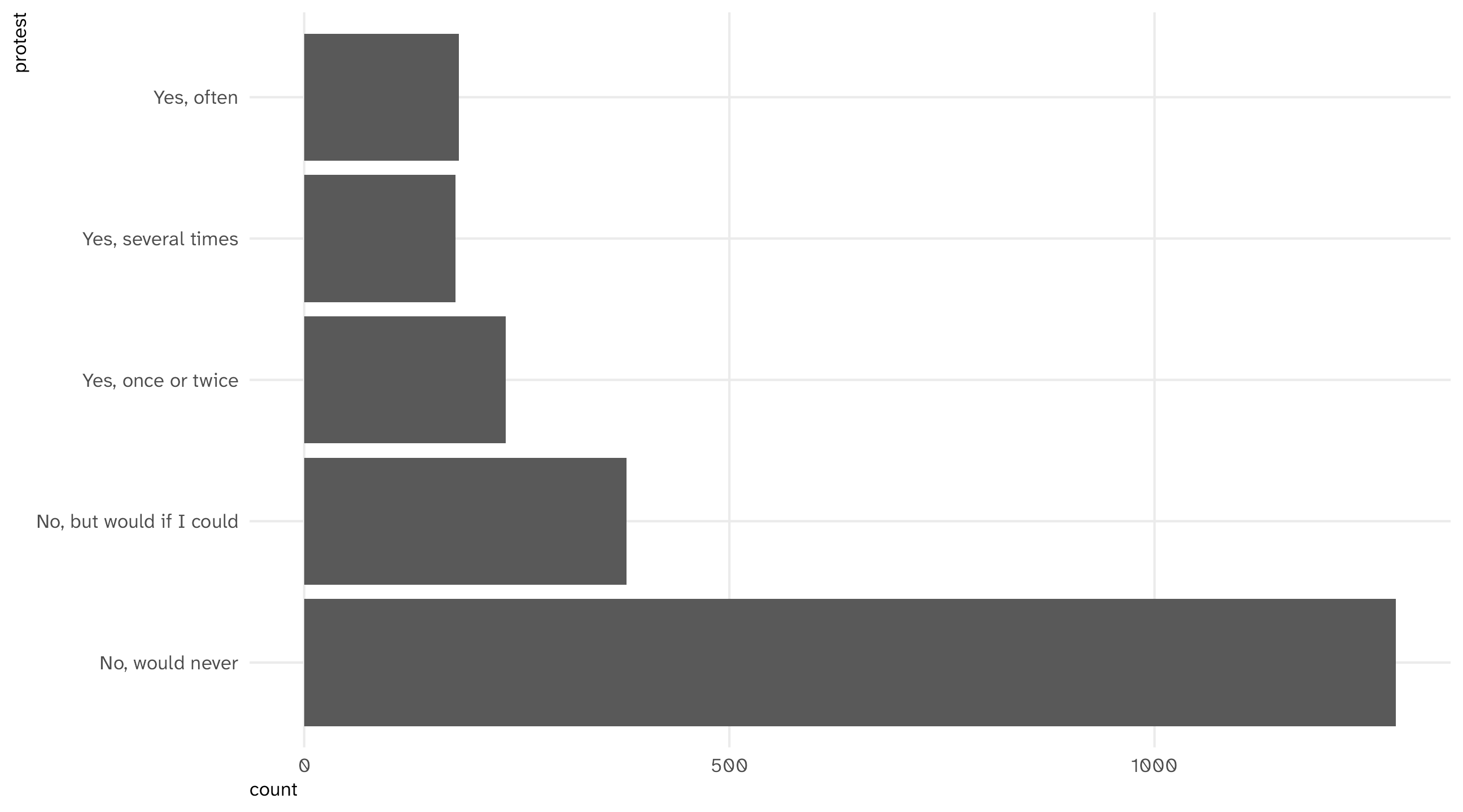
Barplots place a category (an answer, a place, a group) on one axis and a quantity (a count, an average, a share) on the other

Useful for making comparisons, highlighting differences

The grammar of barplots

Afrobarometer, one row per respondent
age region protest
27 Amhara No, would never
66 Amhara No, would never
25 Oromia No, would never
19 Amhara Yes, once or twice
25 Oromia No, would never
Mapping the data
Data Aesthetic Geometry
protest y geom_bar()


geom_bar() counts the rows in each category for you, like geom_histogram() does for bins. (If you already have the numbers, geom_col() plots them as they are)

Note

You could put the category on the x-axis instead, but I think categories look better on the y-axis

The barplot

Code
ggplot(protest, aes(y = protest)) + 
  geom_bar()

Where do you draw the line?

Five answers is often too many. We want two: protester or not. But where’s the line?
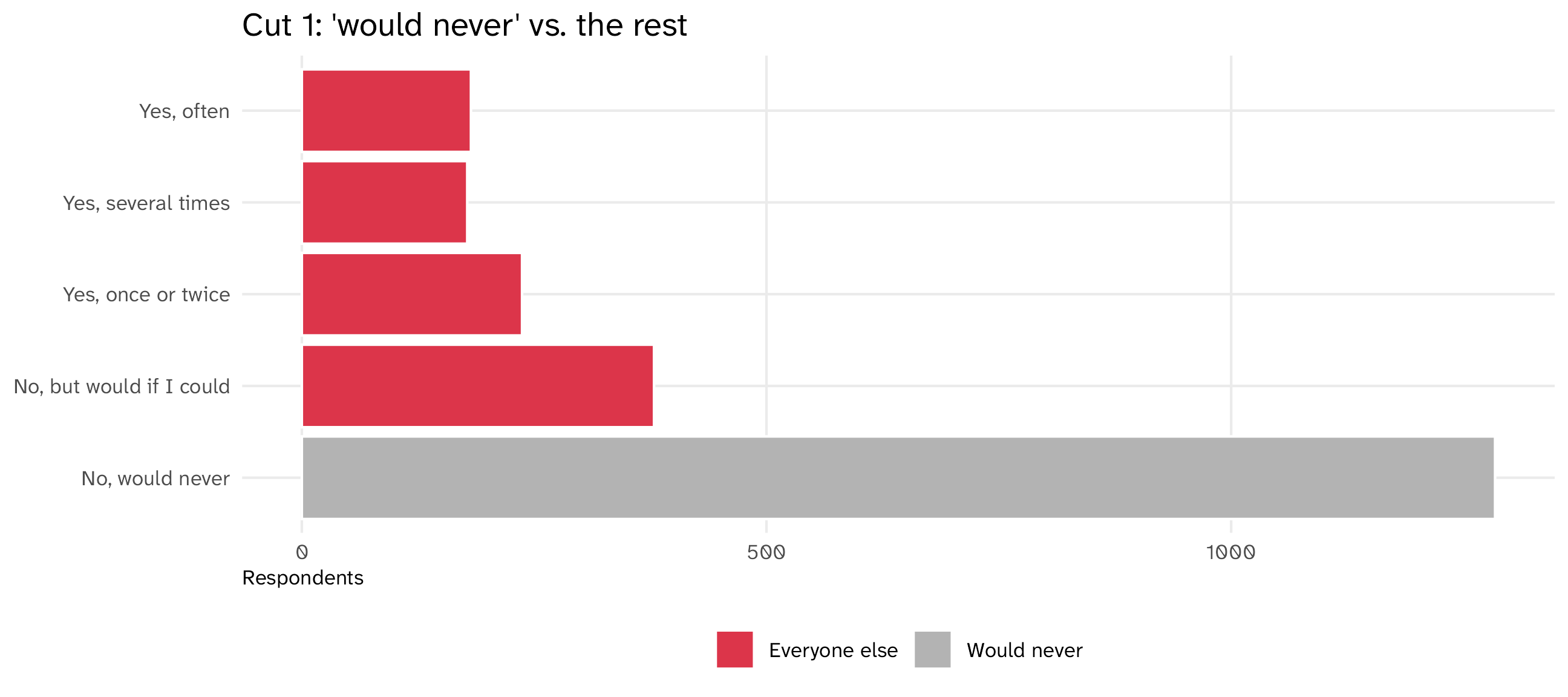
Cut 1 lumps people who would protest in with people who did. Cut 2 separates the two “no” answers from the three “yes” answers. Each “yes” bar is small alone; together they’re a quarter of the sample. Read the labels and the counts before you cut (Day 2: case_when() makes the cut)

The four graphs

Graph aes() geom_ To show... To look for...
Scatterplot x = cause, y = effect point() a relationship outliers, curves
Time series x = date, y = variable line() a trend cliffs, gaps, jumps
Histogram x = cont. variable histogram() a distribution skew, impossible values
Barplot y = category bar() a comparison missing, tiny groups, where to cut

Same four graphs, two jobs. Know how and when to use which!

There’s always more

For all the graphs I showed you today, there are many more variations and options

Check out the large number of dataviz packages online, including:

  • ggridges for ridge plots
  • gganimate for animated plots
  • ggalluvial for alluvial plots
  • waffle for waffle plots

This afternoon

Problem set 1

Inside your camp project, write code/01_set.R that makes the graphs in the problem set.

It is your script: for any line in it, you should be able to say what it does.

Nothing is turned in. Your figures/ folder is the record of what you did.