| Move | What changes | Function | When |
|---|---|---|---|
| Keep the rows you want | fewer rows | filter() | today |
| Add new columns | more columns | mutate() | today |
| Save it | a name you can reuse | = | today |
| Pick columns, sort, summarise, combine | columns, order, one row per group, two tables into one | select(), arrange(), summarise(), join() | tomorrow |
Data wrangling I
Quant Camp
September 14, 2026
Plan for today
- Wrangling is a pipeline
filter(): keep the rows you want- Save what you made: objects
mutate(): add new columns- The whole pipeline in one script
Wrangling is a pipeline
What is data-wrangling?
…the process of transforming and mapping data from one “raw” data form into another format with the intent of making it more appropriate and valuable for a variety of downstream purposes such as analytics… Data analysts typically spend the majority of their time in the process of data wrangling compared to the actual analysis of the data. – Wikipedia
Collect raw data \(\rightarrow\) wrangle to usable form \(\rightarrow\) analyze it
Only a few moves
Raw data almost never arrives in the shape you need. Wrangling is the handful of moves that get it there:
Raw data ➜ filter(): keep rows ➜ mutate(): add columns ➜ save it ➜ the table you plot
Today: two moves, and how to save what they make. Tomorrow adds a few more. That’s most of what wrangling is
New starting point
Yesterday, the data was ready and the first step of your code was
ggplot()I did the wrangling (the
filter()in the UN votes script)Today, you will wrangle the data
First step is now the data object
Pipes: connecting data to functions
To wrangle data, we want to link data to functions, using pipes
What are pipes?
What are pipes?
Here, I am taking the dataset big_five from {juanr} and passing it to a series of functions, in order:
group_by(),summarise(),filter(), anddrop_na()
The output from each step gets passed onto the next step
Mental shortcut
You can think about the pipe as if it said “and then”…
Take the data object big_five, AND THEN
group_by country, AND THEN
summarise so that…
Why pipes?
Pipes make code more legible
With pipes:
filter(): keep the rows you want
Raw data ➜ filter(): keep rows ➜ mutate(): add columns ➜ save it ➜ the table you plot
Subsetting data
Subsetting data means selecting a portion of a dataset with certain characteristics
Why do this?
- Sometimes we want to focus on a specific subset of data: the South, Latin America, etc.
- Also useful to deal with common problems: outliers, missing data, strange responses
- A common sanity check: does my data have impossible values?
Our first wrangling function: filter()
filter() subsets data objects based on rules,
filter() drops observations that don’t meet our criteria
Example: subset gapminder for countries in the Americas
# A tibble: 1,704 × 6
  country     continent  year lifeExp      pop gdpPercap
  <fct>       <fct>     <int>   <dbl>    <int>     <dbl>
1 Afghanistan Asia       1952    28.8  8425333      779.
2 Afghanistan Asia       1957    30.3  9240934      821.
3 Afghanistan Asia       1962    32.0 10267083      853.
4 Afghanistan Asia       1967    34.0 11537966      836.
5 Afghanistan Asia       1972    36.1 13079460      740.
# ℹ 1,699 more rows# A tibble: 300 × 6
country continent year lifeExp pop gdpPercap
<fct> <fct> <int> <dbl> <int> <dbl>
1 Argentina Americas 1952 62.5 17876956 5911.
2 Argentina Americas 1957 64.4 19610538 6857.
3 Argentina Americas 1962 65.1 21283783 7133.
4 Argentina Americas 1967 65.6 22934225 8053.
5 Argentina Americas 1972 67.1 24779799 9443.
# ℹ 295 more rowsGood rule of thumb: notice the changing number of rows
Using filter()
We need to tell R which observations we want to include (or exclude) using rules
Rules rely on logical operators:
- Equal to, not equal to, less than, more than, included in, etc.
- Observations that meet the rule are returned; those that are not are dropped
| Operator | meaning |
|---|---|
| == | equal to |
| != | not equal to |
| > | greater than |
| < | less than |
| >= | greater than or equal to |
| <= | less than or equal to |
| & | AND (both conditions true) |
| | | OR (either condition is true) |
Let’s look at some examples…
Countries in the Americas with low life expectancy
Filter for country-years in the Americas…
# A tibble: 300 × 6
  country   continent  year lifeExp      pop gdpPercap
  <fct>     <fct>     <int>   <dbl>    <int>     <dbl>
1 Argentina Americas   1952    62.5 17876956     5911.
2 Argentina Americas   1957    64.4 19610538     6857.
3 Argentina Americas   1962    65.1 21283783     7133.
4 Argentina Americas   1967    65.6 22934225     8053.
5 Argentina Americas   1972    67.1 24779799     9443.
# ℹ 295 more rowsAnd then with life expectancy lower than 50:
# A tibble: 28 × 6
country continent year lifeExp pop gdpPercap
<fct> <fct> <int> <dbl> <int> <dbl>
1 Bolivia Americas 1952 40.4 2883315 2677.
2 Bolivia Americas 1957 41.9 3211738 2128.
3 Bolivia Americas 1962 43.4 3593918 2181.
4 Bolivia Americas 1967 45.0 4040665 2587.
5 Bolivia Americas 1972 46.7 4565872 2980.
# ℹ 23 more rowsNotice words are in quotations and numbers are not!
Countries not in the Americas
We can also subset by excluding: the ! symbol negates ➡️ not equal to
Countries not in the Americas:
# A tibble: 1,404 × 6
country continent year lifeExp pop gdpPercap
<fct> <fct> <int> <dbl> <int> <dbl>
1 Afghanistan Asia 1952 28.8 8425333 779.
2 Afghanistan Asia 1957 30.3 9240934 821.
3 Afghanistan Asia 1962 32.0 10267083 853.
4 Afghanistan Asia 1967 34.0 11537966 836.
5 Afghanistan Asia 1972 36.1 13079460 740.
# ℹ 1,399 more rowsFilter a range of values
Country-years with at least 20 million people but no more than 100 million
# A tibble: 342 × 6
country continent year lifeExp pop gdpPercap
<fct> <fct> <int> <dbl> <int> <dbl>
1 Afghanistan Asia 1997 41.8 22227415 635.
2 Afghanistan Asia 2002 42.1 25268405 727.
3 Afghanistan Asia 2007 43.8 31889923 975.
4 Algeria Africa 1982 61.4 20033753 5745.
5 Algeria Africa 1987 65.8 23254956 5681.
# ℹ 337 more rowsNotice this is identical to:
# A tibble: 342 × 6
country continent year lifeExp pop gdpPercap
<fct> <fct> <int> <dbl> <int> <dbl>
1 Afghanistan Asia 1997 41.8 22227415 635.
2 Afghanistan Asia 2002 42.1 25268405 727.
3 Afghanistan Asia 2007 43.8 31889923 975.
4 Algeria Africa 1982 61.4 20033753 5745.
5 Algeria Africa 1987 65.8 23254956 5681.
# ℹ 337 more rowsComplex conditions with |
The OR (|) operator: “return observations where this is true OR that is true”
Countries in the Americas OR Europe, with GDP per capita over $30,000
# A tibble: 35 × 6
country continent year lifeExp pop gdpPercap
<fct> <fct> <int> <dbl> <int> <dbl>
1 Austria Europe 2002 79.0 8148312 32418.
2 Austria Europe 2007 79.8 8199783 36126.
3 Belgium Europe 2002 78.3 10311970 30486.
4 Belgium Europe 2007 79.4 10392226 33693.
5 Canada Americas 2002 79.8 31902268 33329.
# ℹ 30 more rowsNote
The | should be above your Return/Enter key
Using filter() to find bad data
Made-up survey of 1,000 adults. The codebook says age is in years. Is it?
A minimum of -99 and a maximum of 999. Nobody is those ages. Write the rule for what should not exist and look at what comes back:
Those are missing-value codes (-99 “refused”, 999 “don’t know”), not ages. The codebook knew; the data file didn’t say
…and to remove it
Flip the rule around: keep the rows that should exist, and save the result under a new name
16 rows gone
Same move for any variable with rules: turnout over 100%, income below zero, a year before the survey existed. Filter to find it, filter to drop it, count the difference
Read before you run
This is how you’ll read the agent’s wrangling code all week. Before running it, ask: what should come out?
- How many rows, roughly? More or fewer than the 142 countries in 2007?
- Which countries would you bet are in there?
# A tibble: 13 × 6
country continent year lifeExp pop gdpPercap
<fct> <fct> <int> <dbl> <int> <dbl>
1 Australia Oceania 2007 81.2 20434176 34435.
2 Canada Americas 2007 80.7 33390141 36319.
3 France Europe 2007 80.7 61083916 30470.
4 Hong Kong, China Asia 2007 82.2 6980412 39725.
5 Iceland Europe 2007 81.8 301931 36181.
# ℹ 8 more rows🚨 Your turn: the (unusual) American voter 🚨
Here’s data of real voters from the Cooperative Election Study:
| state | sex | age | educ | race | pid7 | ideo5 | religion | votechoice | hispanic | know_governor | conceal | prochoice | cleanair | wall | mandmin | aca | minwage | newsint |
|---|---|---|---|---|---|---|---|---|---|---|---|---|---|---|---|---|---|---|
| Minnesota | Female | 63 | Some college | White | Strong Democrat | Moderate | Roman Catholic | Joe Biden (Democrat) | No | Democrat | Oppose | Oppose | Support | Oppose | Support | Oppose | Favor | Most of the time |
| Virginia | Female | 70 | 4-year | White | Strong Republican | Very conservative | Roman Catholic | Donald J. Trump (Republican) | No | Democrat | Support | Oppose | Oppose | Support | Support | Support | Oppose | Most of the time |
| Florida | Male | 58 | 2-year | White | Independent | Moderate | Nothing in particular | Joe Biden (Democrat) | No | Republican | Oppose | Support | Support | Oppose | Support | Oppose | Oppose | Some of the time |
| Utah | Female | 23 | High school graduate | White | Independent | Not sure | Nothing in particular | NA | No | Not sure | Oppose | Support | Support | Oppose | Support | Oppose | Favor | Some of the time |
| New York | Male | 68 | 4-year | White | Strong Democrat | Very liberal | Nothing in particular | Joe Biden (Democrat) | No | Democrat | Oppose | Support | Support | Oppose | Support | Oppose | Favor | Most of the time |
🚨 Your turn: the (unusual) American voter 🚨
Using bot, write a filter() that finds the most unusual American voter you can think of. How many rows come back?
Then ask your agent to find a voter even more unusual than yours. Read the filter() it wrote: what did it decide “unusual” means?
Note
data |> distinct(variable) returns a variable’s unique values
Save what you made: objects
Raw data ➜ filter(): keep rows ➜ mutate(): add columns ➜ save it under a name ➜ the table you plot
Preview, Save As, Save
Every line of wrangling does one of three things you already know from every app on your computer:
| What you type | What it is | What happens |
|---|---|---|
| gapminder |> filter(continent == "Americas") | Preview | R shows you the result, then throws it away |
| gap_americas = gapminder |> filter(...) | Save As | A new object; the original is untouched |
| gapminder = gapminder |> filter(...) | Save | The original is replaced |
The = is the save button. No =, nothing saved
Preview: R throws it away
When you wrangle data, you are modifying it; but those modifications are not stored anywhere:
# A tibble: 300 × 6
  country   continent  year lifeExp      pop gdpPercap
  <fct>     <fct>     <int>   <dbl>    <int>     <dbl>
1 Argentina Americas   1952    62.5 17876956     5911.
2 Argentina Americas   1957    64.4 19610538     6857.
3 Argentina Americas   1962    65.1 21283783     7133.
4 Argentina Americas   1967    65.6 22934225     8053.
5 Argentina Americas   1972    67.1 24779799     9443.
# ℹ 295 more rowsNow try to use that result on the next line:
Error: object 'gap_americas' not found“Object not found” means: you never saved anything by that name. R showed you the filtered rows and forgot them
Save As: give it a name
To store the modified data, we need to assign the output to an object. I’ll call my new object gap_americas:
Two steps:
- come up with a name for the object (e.g.,
gap_americas) - use the assignment operator (
=or<-) to assign the modified data to that name
Notice that nothing printed. To see what you saved, type its name:
# A tibble: 300 × 6
  country   continent  year lifeExp      pop gdpPercap
  <fct>     <fct>     <int>   <dbl>    <int>     <dbl>
1 Argentina Americas   1952    62.5 17876956     5911.
2 Argentina Americas   1957    64.4 19610538     6857.
3 Argentina Americas   1962    65.1 21283783     7133.
4 Argentina Americas   1967    65.6 22934225     8053.
5 Argentina Americas   1972    67.1 24779799     9443.
# ℹ 295 more rowsWatch the Environment pane
The Environment pane (top right in RStudio) lists every object you’ve saved. Before you run each line, predict: does something appear up there?
| Environment | |
|---|---|
| gapminder | 1704 obs. of 6 variables |
| gap_americas | 300 obs. of 6 variables |
Line 1 prints and saves nothing. Line 3 prints nothing and saves gap_americas. The pane is how you check what exists
Using our new object
We can then use our new object:
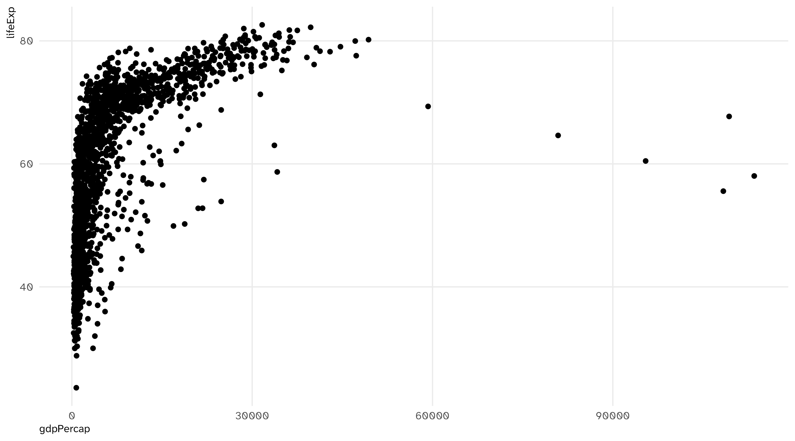
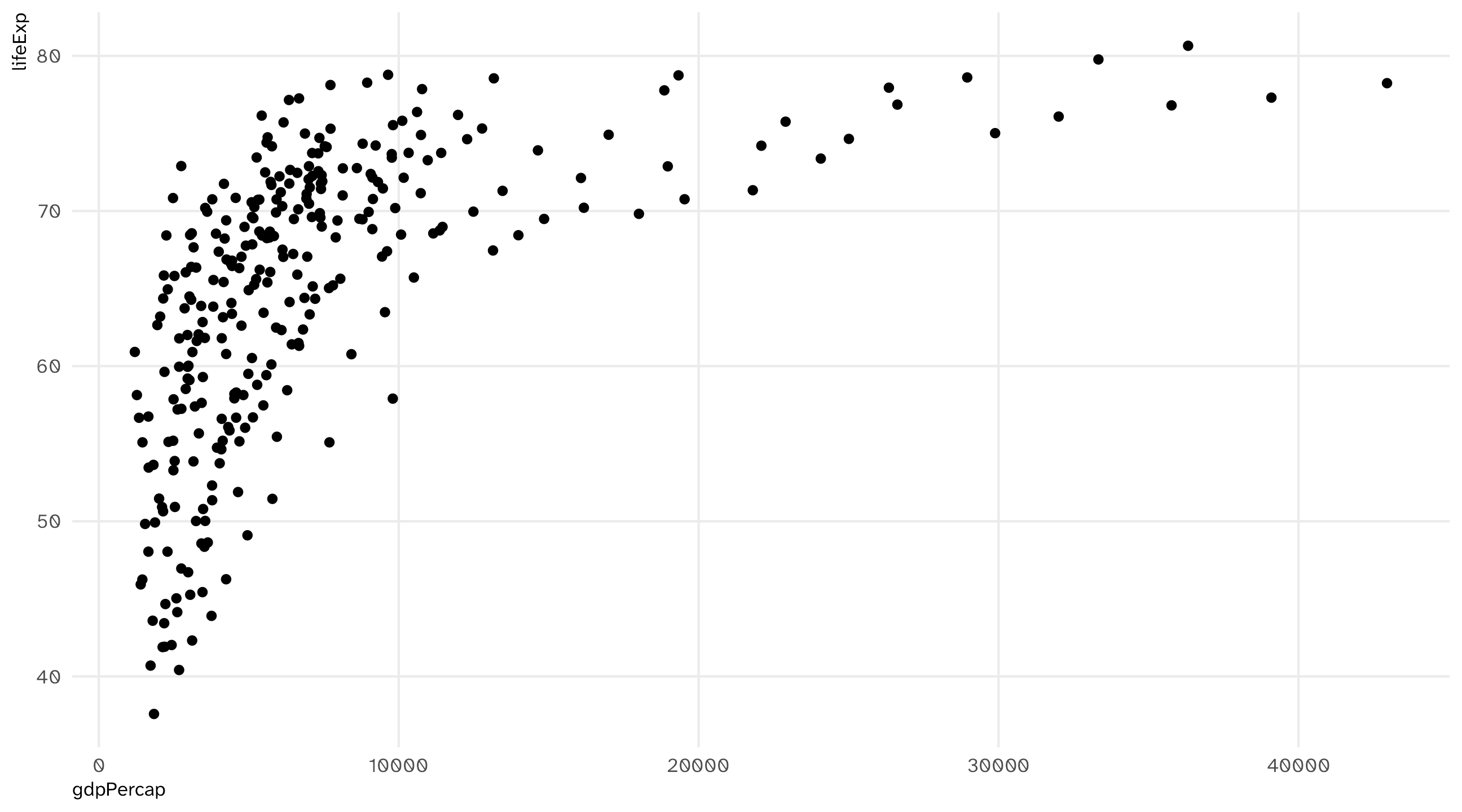
Notice that the original data is unchanged!
Naming objects
There are only two hard things in Computer Science: cache invalidation and naming things. – Phil Karlton
Recommend: keep it short, easy to type, informative, and use _ to separate words
The agent is good at this (un_yes, top_country in yesterday’s organ code). Read its names: they tell you what it thinks the object is
Save: overwrite the original
You can overwrite the original object by making the “new” object name the same as the old one
With filter() this is often a bad idea, since you “lose” the original data and might want it back. (I do, so I’m putting it back now)
🚨 Your turn: predict the environment 🚨
Five lines. Before running them, write down: after line 5, which objects exist in your Environment, and how many rows does each have?
Now run them, one at a time, watching the Environment pane. Were you right?
Then ask the agent: “what is the difference between line 1 and line 2?” Does its answer match yours?
mutate(): add new columns
Raw data ➜ filter(): keep rows ➜ mutate(): add columns ➜ save it ➜ the table you plot
Most violent cities in America?
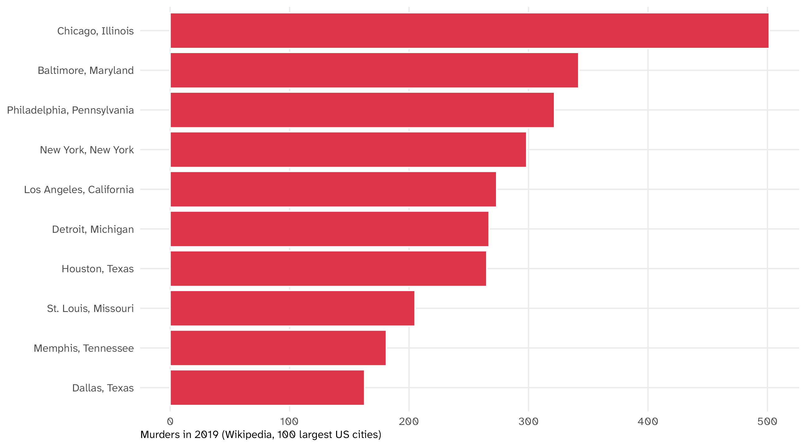
Chicago tops the list, with New York, Philadelphia, Houston, and Los Angeles not far behind. But those are also the biggest cities: more people, more of everything, murders included
Compare rates, not counts
To compare cities fairly we normalize: divide by population, so every city is on the same footing
\(\text{Murders per person} = \frac{\text{Murders}}{\text{Population}}\), which is a tiny number, so by convention we scale it up:
\(\text{Murder rate per 100,000} = \frac{\text{Murders}}{\text{Population}} \times 100{,}000\)
The same move shows up everywhere: GDP per capita, cases per million, votes per registered voter. Counts tell you about size; rates let you compare
Comparing murder rates
If we look at murder rates, the picture changes:
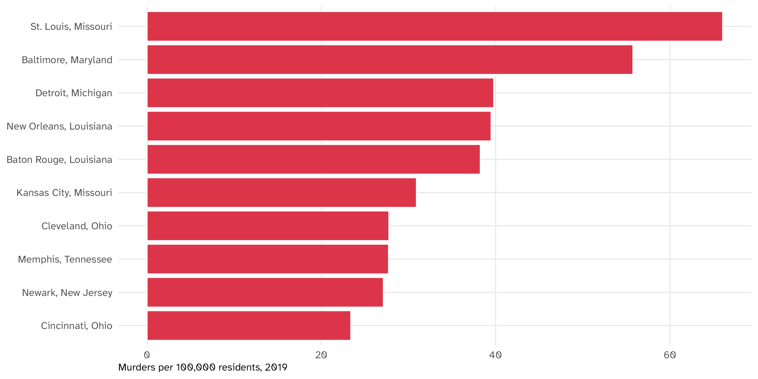
That rate column is not in my data. I have to make it: that’s mutate()
Creating new variables using mutate
This rate variable is not in my data, I need to create it using mutate()
Using mutate
Using mutate
# A tibble: 100 × 5
  state   city      population murder_total murder_capita
  <chr>   <chr>          <dbl>        <dbl>         <dbl>
1 Alabama Mobile        248431        50.0      0.000201
2 Alaska  Anchorage     296188        27.0      0.0000912
3 Arizona Chandler      249355         5.01     0.0000201
4 Arizona Gilbert       242090         5.01     0.0000207
5 Arizona Glendale      249273        12.0      0.0000481
# ℹ 95 more rows
Notice that I named a new variable, murder_capita
Using mutate
# A tibble: 100 × 6
  state   city      population murder_total per_capita  rate
  <chr>   <chr>          <dbl>        <dbl>      <dbl> <dbl>
1 Alabama Mobile        248431        50.0   0.000201  20.1
2 Alaska  Anchorage     296188        27.0   0.0000912  9.12
3 Arizona Chandler      249355         5.01  0.0000201  2.01
4 Arizona Gilbert       242090         5.01  0.0000207  2.07
5 Arizona Glendale      249273        12.0   0.0000481  4.81
# ℹ 95 more rows
Notice the new columns
Save As, or Save?
As with filter(), you can Save As (a new object):
Or Save (overwrite the old one):
Q: When should you make a new object, or overwrite an old one?
Save As, or Save?
In general, overwriting is fine when you are adding stuff to your data (as with mutate())
# A tibble: 100 × 8
  state city  population murder_total per_capita  rate murder_capita murder_rate
  <chr> <chr>      <dbl>        <dbl>      <dbl> <dbl>         <dbl>       <dbl>
1 Alab… Mobi…     248431        50.0   0.000201  20.1      0.000201        20.1
2 Alas… Anch…     296188        27.0   0.0000912  9.12     0.0000912        9.12
3 Ariz… Chan…     249355         5.01  0.0000201  2.01     0.0000201        2.01
4 Ariz… Gilb…     242090         5.01  0.0000207  2.07     0.0000207        2.07
5 Ariz… Glen…     249273        12.0   0.0000481  4.81     0.0000481        4.81
# ℹ 95 more rows
This is because you are not losing information, only adding
New column, or overwrite the old one?
If the new variable has the same name as the old one, you will overwrite it; This is sometimes a bad idea since you lose the original data
This is confusing because murder_total is no longer a total, it’s a proportion
# A tibble: 100 × 3
  state   city      murder_total
  <chr>   <chr>            <dbl>
1 Alabama Mobile       0.000201
2 Alaska  Anchorage    0.0000912
3 Arizona Chandler     0.0000201
4 Arizona Gilbert      0.0000207
5 Arizona Glendale     0.0000481
# ℹ 95 more rowsThe double-run trap
Say I want population in thousands, and I overwrite the column with itself:
Run it once:
# A tibble: 3 × 2
  city      population
  <chr>          <dbl>
1 Mobile          248.
2 Anchorage       296.
3 Chandler        249.
Hit Cmd + Enter on the same line again, by accident:
# A tibble: 3 × 2
  city      population
  <chr>          <dbl>
1 Mobile         0.248
2 Anchorage      0.296
3 Chandler       0.249
No error. Mobile now has 0.25 “thousand” people. Every rate you compute from here is wrong, silently
This is why a script runs top to bottom from a fresh session: each line runs exactly once
Start fresh
Look at your Environment pane right now. How many objects are in it? Which ones did today’s script make, and which are left over from yesterday, another class, another project?
Leftovers are dangerous: your script seems to work because an object from yesterday happens to exist. On a fresh computer, it fails
The habit, every time you think you’re done:
- Restart R: Session ▸ Restart R (Cmd/Ctrl + Shift + F10). Watch the Environment pane empty
- Run the script top to bottom: Cmd/Ctrl + Shift + Enter, or click Source
If it runs after a restart, it’s real. If it doesn’t, you found the bug before it found you
Never restore the mess
Once, today: Tools ▸ Global Options ▸ General
- Uncheck Restore .RData into workspace at startup
- Set Save workspace to .RData on exit to Never
Now nothing carries over between sessions unless a script makes it
Delegate the check. Ask the agent: “Run code/02_set.R from a fresh R session and tell me whether it errors.” When the agent runs a script it starts a brand-new R every time, so this is the same test. Then read what it reports
Your CLAUDE.md already says every script must run top to bottom from a fresh R session. That rule was written for the agent. It’s yours now too
When to Save As, when to Save
| You are... | Example | Do this | Why |
|---|---|---|---|
| removing rows | filter(year == 2007) | Save As (new name) | you may want the rows back |
| adding columns | mutate(rate = murders / pop) | Save (overwrite) is fine | nothing is lost, only added |
| replacing a column with itself | mutate(pop = pop / 1000) | stop and think; prefer a new column name | the old values are gone, and running it twice breaks it |
And whichever you choose: look at the Environment pane afterwards. Is the object there? Does the row count make sense?
🚨 Your turn 🌡️ Climate change 🌡️ 🚨
Using climate, make the following two plots looking only at USA, China, India. Save each wrangling step under a name before you plot it:
A grouped time-series of co2 emissions over time (separate country by color)
A grouped time-series of co2 emissions per capita over time (separate country by color). Check
?climate: what unit isco2in?Who’s to “blame” for climate change? And where should we focus environmental efforts?
The whole pipeline in one script
Raw data ➜ filter(): keep rows ➜ mutate(): add columns ➜ save it ➜ the table you plot
The pipeline you just built
Look at what you just did in the climate exercise. It’s the diagram from this morning:
# keep three countries
big_three = climate |>
  filter(country == "United States" | country == "China" | country == "India")

# new column: co2 is in million tonnes, so this is tonnes per person
big_three = big_three |>
  mutate(co2_per_capita = co2 / population * 1e6)

# the table you plot
ggplot(big_three, aes(x = year, y = co2_per_capita, color = country)) +
  geom_line(linewidth = 1.2) +
  labs(x = NULL, y = "CO2 per person (tonnes)", color = NULL)

ggsave(here("figures", "co2_per_capita.png"), width = 8, height = 5)
Most wrangling you do this year will have this shape, just with more steps in the middle
Where does the file go?
A file path is an address. There are two kinds
Absolute: starts at the root of your computer. Only works on your computer
Relative: starts from the folder R is working in. Inside an RStudio project, that’s the project folder, on any computer
Relative paths are why the project matters: whoever opens rproject_camp.Rproj (you next month, a coauthor, the agent) starts from the same place
here() builds the path for you
here() finds your project folder (it looks for the .Rproj file) and builds the path from there:
[1] "/Users/juan/Desktop/rproject_camp/data/clean/big_three.rds"- Each piece is one folder or file name;
here()adds the slashes, correctly for Mac and Windows - The printed path is different on every computer. The code is the same
This is why the agent writes here("figures", ...) and never /Users/you/...: your CLAUDE.md tells it to. Do the same
Save the clean data
You often want to save your clean data to a file, so you can use it later without having to re-run all your wrangling code
You can use write_* functions from {readr}, where what replaces * depends on the file type
For common use (e.g., opening in Excel), saving to .csv is a good idea
For working within R, .rds is nice
Raw data goes in data/. Clean data goes in data/clean/. Never save over the raw file
A good script
code/02_co2.R
# CO2 per person in the US, China, and India ---------------------------------

# libraries
library(tidyverse)
library(juanr)
library(here)

# look at the raw data (one row per country-year)
climate

# wrangle
big_three = climate |>
  # keep three countries
  filter(country == "United States" | country == "China" | country == "India") |>
  # co2 is in million tonnes; this is tonnes per person
  mutate(co2_per_capita = co2 / population * 1e6)

# save the clean data
write_rds(big_three, here("data", "clean", "big_three.rds"))

# plot and save the plot
ggplot(big_three, aes(x = year, y = co2_per_capita, color = country)) +
  geom_line(linewidth = 1.2) +
  labs(x = NULL, y = "CO2 per person (tonnes)", color = NULL)

ggsave(here("figures", "co2_per_capita.png"), width = 8, height = 5)
Directing the agent is describing the pipeline
I asked the agent two versions of the same question:
Vague: “using the climate data from juanr, who is to blame for climate change?”
. . .
130 lines. It picked three definitions of “blame”, the year 2020, and dropped every country under a million people. It chose all of that for me
Precise: “Using climate (one row per country-year; co2 in million tonnes): keep the US, China, and India, compute CO2 per person in tonnes, and plot it over time by country. Save to figures/. Comment the code.”
. . .
18 lines. The pipeline you just wrote, with a filter() and a mutate() you can read
A good request is the pipeline in words: the data, what a row is, which rows to keep, what to compute, what comes out
This afternoon
Problem set 2
Inside your camp project, write code/02_set.R that answers the questions in the problem set.
It is your script: for any line in it, you should be able to say what it does.
New today: for every filter(), say how many rows it dropped. For every mutate(), say what unit the new column is in. For every =, say what’s in the object.
When you think you’re done: restart R and run the script top to bottom. If it works then, it works.
Nothing is turned in. Your figures/ and data/clean/ folders are the record of what you did.