# A tibble: 7 × 2
  ideo5                 n
  <fct>             <int>
1 Very liberal       8132
2 Liberal           11331
3 Moderate          19226
4 Conservative      10716
5 Very conservative  6803
6 Not sure           4752
7 <NA> 40Data Wrangling II
Quant Camp
September 15, 2026
Plan for today
- Working with strings
- Merging data
- Long and wide data
Three problems
Yesterday, and today
Yesterday: keep the rows you want, add the columns you need, save what you made, put it all in one script
Today, three problems real data throws at you:
The data is finer than you need. You don’t care about the distinction between “Very liberal” and “Liberal”, but that’s how the data is stored.
The data is in two tables. Democracy scores in one, trade in another. You need both.
The data is the wrong shape. One column per year, when you need one row per year.
Working with strings
Values are text, and text is messy
Before you clean a column, look at what’s in it. count() shows every value and how often it appears:
What if instead of all these categories, we wanted something simpler: conservatives, liberals, and other?
Functions for text: str_*()
There’s a whole family of functions for text (“strings”), all starting with str_
Three do most of the work:
| Function | What it does |
|---|---|
str_detect(VARIABLE, PATTERN) |
Is PATTERN in VARIABLE? TRUE or FALSE |
str_replace(VARIABLE, OLD, NEW) |
Swap OLD for NEW |
str_remove(VARIABLE, PATTERN) |
Delete PATTERN |
They all go inside filter() or mutate(), like everything else
Finding text: str_detect()
str_detect() returns TRUE or FALSE, so it slots right into filter()
parties has one row per European party. No two Green parties share a name, so == can’t find them. A pattern can:
# A tibble: 53 × 3
  country     party                                  family
  <chr>       <chr>                                  <chr>
1 Australia   Australian Greens                      Green/Ecologist
2 Austria     The Greens -- The Green Alternative    Green/Ecologist
3 Austria     United Greens Austria                  Green/Ecologist
4 Belgium     Agalev -- Green                        Green/Ecologist
5 Bulgaria    Green Party of Bulgaria                Green/Ecologist
6 Canada      Green Party of Canada                  Green/Ecologist
7 Switzerland Feminists and Green-Alternative Groups Green/Ecologist
# ℹ 46 more rows
53 parties in 31 countries, in one line
Check the pattern
A pattern is a guess. parties also has a hand-coded family column, so we can check the guess:
# A tibble: 6 × 2
  family                  n
  <chr>               <int>
1 Green/Ecologist        47
2 Liberal                 2
3 Agrarian                1
4 Communist/Socialist     1
5 Social democracy        1
6 no family               1
Six aren’t Green parties at all. Why? “Solidarity (Greenland)”
And 39 Green parties have no “Green” in their name (“Ecoglasnost”). Check a pattern against something you trust
Replacing text: str_replace()
Sometimes a value is spelled one way and you need it spelled another
str_replace(VARIABLE, OLD, NEW) swaps OLD for NEW. For example, be respectful of Türkiye:
# A tibble: 12 × 6
  country continent  year lifeExp      pop gdpPercap
  <chr>   <fct>     <int>   <dbl>    <int>     <dbl>
1 Türkiye Europe     1952    43.6 22235677     1969.
2 Türkiye Europe     1957    48.1 25670939     2219.
3 Türkiye Europe     1962    52.1 29788695     2323.
4 Türkiye Europe     1967    54.3 33411317     2826.
5 Türkiye Europe     1972    57.0 37492953     3451.
6 Türkiye Europe     1977    59.5 42404033     4269.
7 Türkiye Europe     1982    61.0 47328791     4241.
# ℹ 5 more rows
Removing text: str_remove()
Say we don’t care about the difference between “Very liberal” and “Liberal”
str_remove(VARIABLE, PATTERN) deletes PATTERN. Remove “Very” and the two collapse into one:
# A tibble: 7 × 3
  ideo5             ideo3            n
  <fct>             <chr>        <int>
1 Very liberal      liberal       8132
2 Liberal           Liberal      11331
3 Moderate          Moderate     19226
4 Conservative      Conservative 10716
5 Very conservative conservative  6803
6 Not sure          Not sure      4752
7 <NA>              <NA>            40
Check your work
Look again at that output. “Very liberal” became “liberal”, with a lowercase l
To R, “liberal” and “Liberal” are still two different words. We didn’t collapse anything
str_replace() to fix the capitalization, once for each side:
Count before, count after. You only know the cleaning worked if you look
Groups from numbers: case_when()
Often the values aren’t text at all. They’re numbers, and we want groups: rich and poor, young and old, Republican-leaning and Democrat-leaning
case_when() does this. It goes inside mutate()
Like filter(), it runs on conditions: case_when(CONDITION ~ LABEL)
If CONDITION is true, assign LABEL
Who won the county?
| name | state | hh_income | per_gop_2020 | per_dem_2020 |
|---|---|---|---|---|
| Vilas County | WI | 40833 | 0.60 | 0.38 |
| Noble County | OH | 38290 | 0.81 | 0.18 |
| Iron County | MO | 36387 | 0.78 | 0.21 |
| Chester County | SC | 33103 | 0.55 | 0.44 |
| Hutchinson County | TX | 44731 | 0.88 | 0.11 |
| Wise County | VA | 36218 | 0.80 | 0.19 |
| Berrien County | MI | 43633 | 0.53 | 0.45 |
| Johnson County | MO | 47223 | 0.67 | 0.30 |
| Fort Bend County | TX | 85297 | 0.44 | 0.55 |
| Turner County | GA | 28326 | 0.62 | 0.37 |
Two vote shares per county. We want to know: who won?
Who won the county?
Start with one condition:
# A tibble: 3,152 × 6
  name           state hh_income per_gop_2020 per_dem_2020 who_won
  <chr>          <chr>     <dbl>        <dbl>        <dbl> <chr>
1 Autauga County AL        53682        0.714       0.270  Republicans
2 Baldwin County AL        50221        0.762       0.224  Republicans
3 Barbour County AL        32911        0.535       0.458  Republicans
4 Bibb County    AL        36447        0.784       0.207  Republicans
5 Blount County  AL        44145        0.896       0.0957 Republicans
# ℹ 3,147 more rows
Rows that match no condition get NA. Look at the Democratic counties
Who won the county?
Add a second condition, separated by a comma:
# A tibble: 3,152 × 6
  name           state hh_income per_gop_2020 per_dem_2020 who_won
  <chr>          <chr>     <dbl>        <dbl>        <dbl> <chr>
1 Autauga County AL        53682        0.714       0.270  Republicans
2 Baldwin County AL        50221        0.762       0.224  Republicans
3 Barbour County AL        32911        0.535       0.458  Republicans
4 Bibb County    AL        36447        0.784       0.207  Republicans
5 Blount County  AL        44145        0.896       0.0957 Republicans
# ℹ 3,147 more rows
How would I add a condition for a (theoretical) tie?
Store it, then check it
Save the result as a new object, then count() the new column:
# A tibble: 2 × 2
  who_won         n
  <chr>       <int>
1 Democrats     557
2 Republicans  2595
No ties, no NA. Every county landed somewhere
Plot it
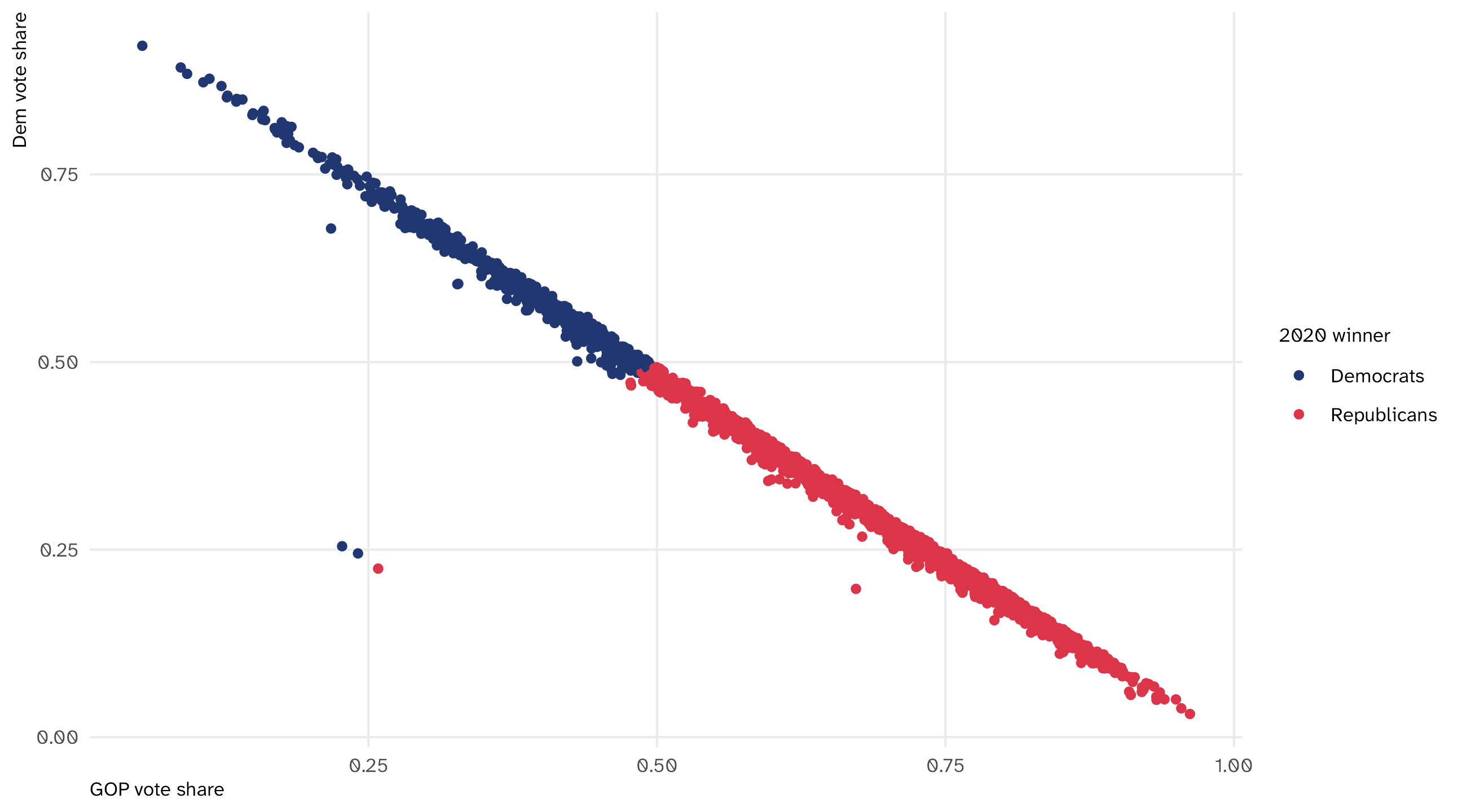
What’s up with those points?
Most points sit on a line: the two shares add up to about 1. Three don’t
To find them, sort. Make the sum a column, then slice_min() grabs the smallest values:
# A tibble: 3 × 7
  name  state hh_income per_gop_2020 per_dem_2020 who_won     total
  <chr> <chr>     <dbl>        <dbl>        <dbl> <chr>       <dbl>
1 <NA>  <NA>         NA        0.227        0.254 Democrats   0.482
2 <NA>  <NA>         NA        0.258        0.225 Republicans 0.483
3 <NA>  <NA>         NA        0.241        0.245 Democrats   0.486
Three rows with no name and no state. Yesterday’s move: filter() them out
🚨 Your turn: three parties 🚨
The pid7 column in bot has seven kinds of partisan. Run count(bot, pid7) to see them
Make a new column,
party3, with three values: “Democrat”, “Republican”, and “Independent / other”.Run
count(pid7, party3). Did every value land where you wanted?Ask your agent to do the same for
ideo5: liberal, moderate, conservative. Read thecase_when()it wrote. Where did it put “Not sure”? If there’s a line you don’t recognize, ask it what that line does
Two tables
The data you need is in two places
Often, the variables you want live in different datasets:
vdem has democracy scores over time
| country | year | v2x_libdem |
|---|---|---|
| Afghanistan | 1789 | 0.02 |
| Afghanistan | 1790 | 0.02 |
| Afghanistan | 1791 | 0.02 |
trade has exports over time
| country | year | exports |
|---|---|---|
| United States of America | 1946 | 9775 |
| United States of America | 1947 | 15369 |
| United States of America | 1948 | 12470 |
I want to plot democracy against exports. Which dataset goes in ggplot()?
Identifiers: what makes a row a row
We can merge two datasets if they share identifier variables
An identifier uniquely picks out each observation. Here, one row is one country in one year:
| country | year | v2x_libdem |
|---|---|---|
| Afghanistan | 1789 | 0.02 |
| Afghanistan | 1790 | 0.02 |
| Afghanistan | 1791 | 0.02 |
| Afghanistan | 1792 | 0.02 |
| Afghanistan | 1793 | 0.02 |
| Afghanistan | 1794 | 0.02 |
| country | year | exports |
|---|---|---|
| United States of America | 1946 | 9775 |
| United States of America | 1947 | 15369 |
| United States of America | 1948 | 12470 |
| United States of America | 1949 | 11920 |
| United States of America | 1950 | 10220 |
| United States of America | 1951 | 14920 |
Both have country and year. Together they identify a row in each dataset
What a merge does
Goal, in words:
- Start with
vdem - Add an
exportscolumn - For each row, look in
tradefor the samecountryandyear, and copy over itsexports - If there’s no match, put
NA
# A tibble: 27,734 × 4
  country      year v2x_libdem exports
  <chr>       <dbl>      <dbl>   <dbl>
1 Afghanistan  1789      0.023      NA
2 Afghanistan  1790      0.023      NA
3 Afghanistan  1791      0.023      NA
4 Afghanistan  1792      0.023      NA
5 Afghanistan  1793      0.023      NA
# ℹ 27,729 more rows
left_join() keeps every row of the first dataset and attaches matching columns from the second
Rule: count rows before and after
A merge is the easiest place to wreck a dataset without any error message
So every time: how many rows before, how many after?
A left_join() should keep the row count of the first dataset. If the number changes, stop
When the key isn’t an identifier
country alone does not identify a row: each country appears in many years
Merge on country alone and R matches every year in vdem to every year in trade for that country:
From 27,734 rows to 1,608,653. No error. Only the count tells you
Plot the result
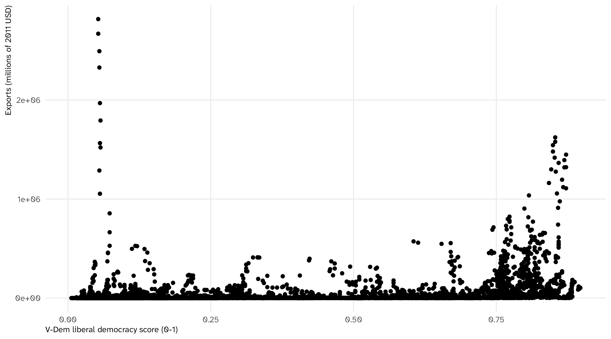
With the merged data, I can plot both variables:
What didn’t merge?
Row counts catch one kind of problem. They miss another: rows that had no match and got NA
anti_join() returns the rows in the first dataset that found no match in the second:
What’s the pattern? The years don’t line up: vdem goes back much further than trade
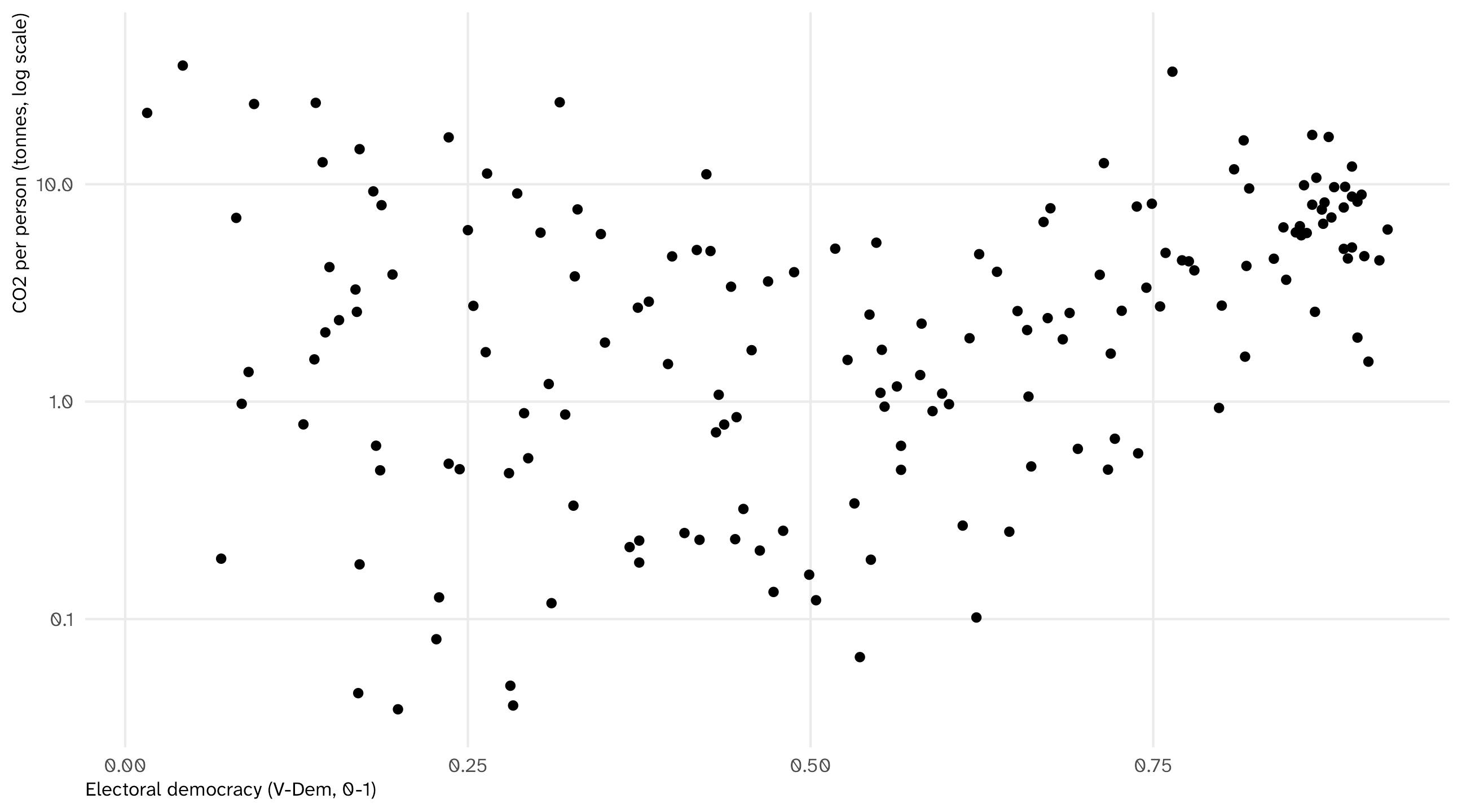
Democracy and emissions
Yesterday’s climate data has CO2. vdem has democracy. Do democracies emit more?
climate_2015 = climate |>
  filter(year == 2015) |>
  select(country, year, population, co2)

vdem_2015 = vdem |>
  filter(year == 2015) |>
  select(country, year, v2x_polyarchy)

dem_co2 = left_join(climate_2015, vdem_2015, by = c("country", "year")) |>
  mutate(co2_pc = co2 * 1e6 / population) # co2 is in million tonnes: tonnes per person

nrow(climate_2015)
[1] 221[1] 221Rows before and after match. Looks fine
Democracy and emissions
Looks fine. Is the United States on this plot?
🚨 Your turn: who’s missing? 🚨
Build
dem_co2as on the slide. Confirm the row counts matchUse
anti_join()to list the countries inclimate_2015that have no democracy score. Find two that surprise youAsk your agent to fix the country names so those two merge, then re-run your
anti_join(). Read what it changed
Text problems become merge problems
# A tibble: 2 × 4
  country        year population   co2
  <chr>         <dbl>      <dbl> <dbl>
1 Turkey         2015   78529416  381.
2 United States  2015  320878304 5372.
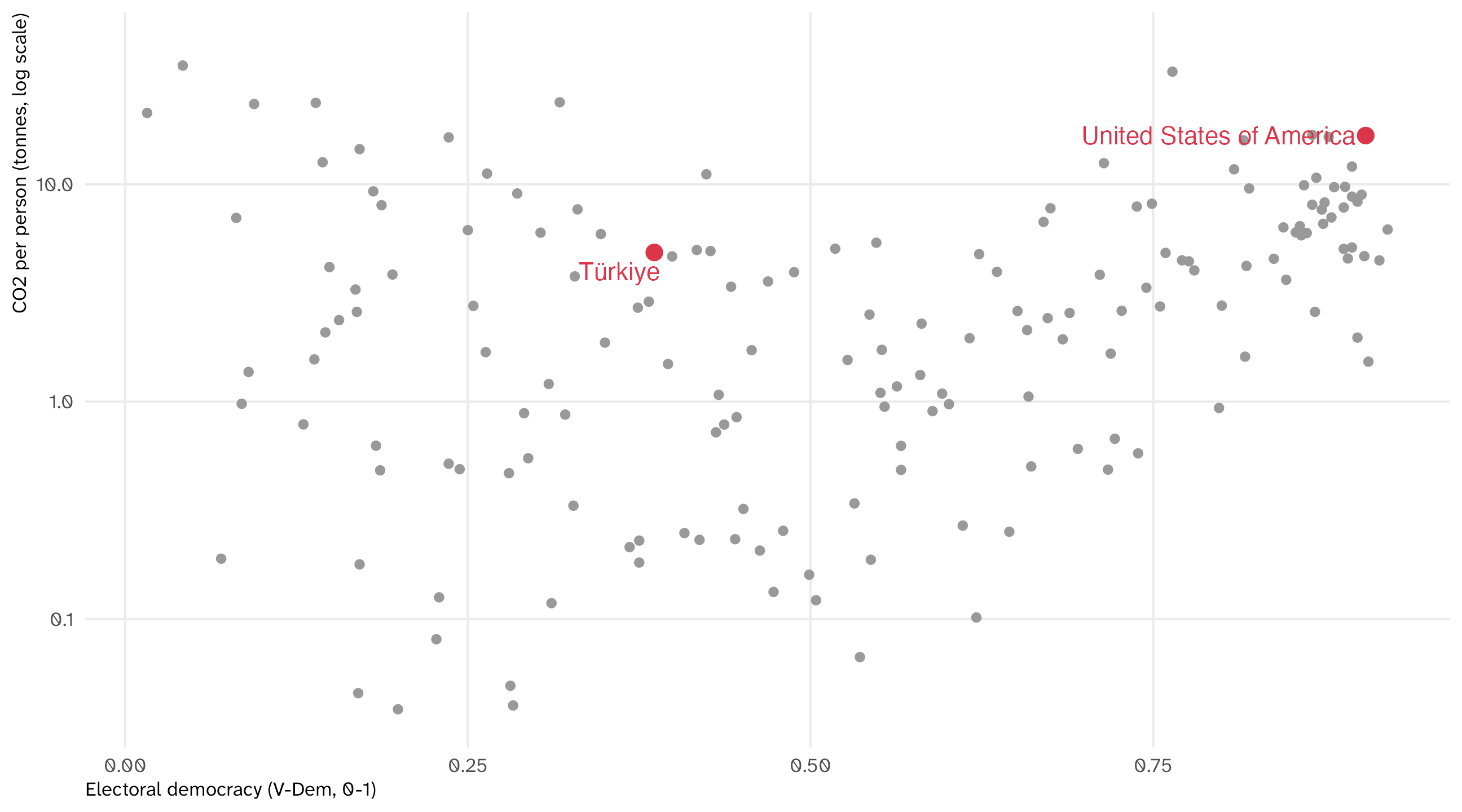
climate says “United States”. vdem says “United States of America”. Same story for “Turkey” and “Türkiye”. No match, no error, no United States on the plot
The fix is the function from this morning:
The United States, restored
Every merge: count rows before and after, then ask what didn’t match
Long and wide
Two shapes for the same data
The same data can be long or wide:
| country | year | lifeExp |
|---|---|---|
| Afghanistan | 1952 | 28.80 |
| Afghanistan | 1957 | 30.33 |
| Afghanistan | 1962 | 32.00 |
| Afghanistan | 1967 | 34.02 |
| Afghanistan | 1972 | 36.09 |
| Afghanistan | 1977 | 38.44 |
| country | 1952 | 1957 | 1962 | 1967 | 1972 | 1977 | 1982 | 1987 | 1992 | 1997 | 2002 | 2007 |
|---|---|---|---|---|---|---|---|---|---|---|---|---|
| Afghanistan | 28.80 | 30.33 | 32.00 | 34.02 | 36.09 | 38.44 | 39.85 | 40.82 | 41.67 | 41.76 | 42.13 | 43.83 |
| Albania | 55.23 | 59.28 | 64.82 | 66.22 | 67.69 | 68.93 | 70.42 | 72.00 | 71.58 | 72.95 | 75.65 | 76.42 |
| Algeria | 43.08 | 45.69 | 48.30 | 51.41 | 54.52 | 58.01 | 61.37 | 65.80 | 67.74 | 69.15 | 70.99 | 72.30 |
| Angola | 30.02 | 32.00 | 34.00 | 35.98 | 37.93 | 39.48 | 39.94 | 39.91 | 40.65 | 40.96 | 41.00 | 42.73 |
| Argentina | 62.48 | 64.40 | 65.14 | 65.63 | 67.06 | 68.48 | 69.94 | 70.77 | 71.87 | 73.28 | 74.34 | 75.32 |
| Australia | 69.12 | 70.33 | 70.93 | 71.10 | 71.93 | 73.49 | 74.74 | 76.32 | 77.56 | 78.83 | 80.37 | 81.24 |
Same numbers. What changed is what a row is
Say the shape you want
The way to describe a shape is to say what one row is:
- Long: “one row per country-year”
- Wide: “one row per country, one column per year”
Long is what ggplot() and most of R want. To plot life expectancy over time, year has to be a column, not fifty column names
Wide is what spreadsheets give you, and what you want to compare two moments: `2007` - `1952` is one line of mutate() in wide data
Some (ahem, World Bank) data arrives wide (one column per year). You will reshape a lot
The functions, so you can ask for them
pivot_longer() goes wide to long. pivot_wider() goes long to wide
# A tibble: 1,704 × 3
  country     year  lifeExp
  <fct>       <chr>   <dbl>
1 Afghanistan 1952     28.8
2 Afghanistan 1957     30.3
3 Afghanistan 1962     32.0
4 Afghanistan 1967     34.0
5 Afghanistan 1972     36.1
# ℹ 1,699 more rows
You don’t need to memorize the arguments. You need to say: “make this long, one row per country-year, with a year column and a lifeExp column.” Then check that the row count makes sense: 142 countries × 12 years = 1,704 rows
This afternoon
Problem set 3
Inside your camp project, write code/03_set.R that answers the questions in the problem set.
It is your script: for any line in it, you should be able to say what it does.
New today: for every case_when(), say which values matched no condition, and what happened to them. For every join, say how many rows before and after, and what didn’t match.
When you think you’re done: restart R and run the script top to bottom. If it works then, it works.
Nothing is turned in. Your figures/ and data/clean/ folders are the record of what you did.