| country | continent | year | lifeExp | pop | gdpPercap |
|---|---|---|---|---|---|
| Afghanistan | Asia | 2007 | 43.83 | 31889923 | 974.58 |
| Albania | Europe | 2007 | 76.42 | 3600523 | 5937.03 |
| Algeria | Africa | 2007 | 72.30 | 33333216 | 6223.37 |
| Angola | Africa | 2007 | 42.73 | 12420476 | 4797.23 |
| Argentina | Americas | 2007 | 75.32 | 40301927 | 12779.38 |
| Australia | Oceania | 2007 | 81.24 | 20434176 | 34435.37 |
Relationships in data
Quant Camp
September 16, 2026
Plan for today
- Summarizing data
- Dummy variables
- Missing data
- Grouped comparisons
- Analyzing categorical data
Summarizing data
Summarizing data
Often, with data, we want to compare things
Are democracies more peaceful than autocracies? Does early voting increase turnout? Are decapitated terrorist groups weaker?
To do this, we often rely on statistical summaries of our data:
Means, medians, minimums, maximums, variances
Summary statistics with summarize()
We can use summarize() to calculate things like the mean, median, etc.
Summarizing condenses data into statistics
| Avg. life exp. | Avg. population | Avg. GDP per capita |
|---|---|---|
| 67.01 | 44021220 | 11680.07 |
Using summarize()
The average life expectancy in the world in 2007:
# A tibble: 1 × 1
  avg_life
     <dbl>
1     67.0
Notice how the data has been summarized; the output is still a table, with only one row
Notice also that I’ve named the summary statistic avg_life, which is now a variable
Using summarize()
I can add more summary statistics, separated by commas:
# A tibble: 1 × 5
  avg_life med_life min_life max_life sd_life
     <dbl>    <dbl>    <dbl>    <dbl>   <dbl>
1     67.0     71.9     39.6     82.6    12.1
Notice how this adds columns to my dataframe
Note
sd() = standard deviation
We can use summary functions in filter()
Which countries had above-average GDP but below-average health?
# A tibble: 3 × 6
  country           continent  year lifeExp     pop gdpPercap
  <fct>             <fct>     <int>   <dbl>   <int>     <dbl>
1 Botswana          Africa     2007    50.7 1639131    12570.
2 Equatorial Guinea Africa     2007    51.6  551201    12154.
3 Gabon             Africa     2007    56.7 1454867    13206.
These are the “outlier” countries from the plot on the first day of class!
We can use summary functions in mutate()
We can also use summary functions in mutate() to create new variables
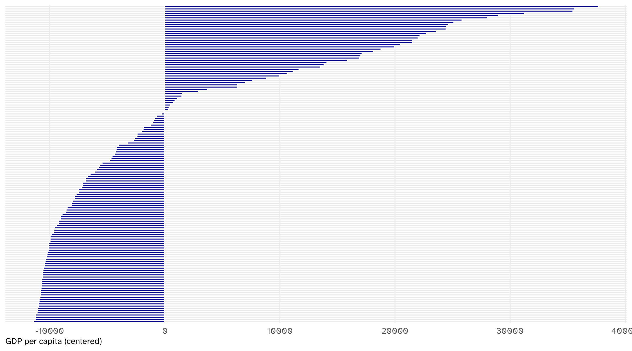
Centering = subtracting the mean from each observation
# A tibble: 142 × 3
  country     gdpPercap gdp_center
  <fct>           <dbl>      <dbl>
1 Afghanistan      975.    -10705.
2 Albania         5937.     -5743.
3 Algeria         6223.     -5457.
4 Angola          4797.     -6883.
5 Argentina      12779.      1099.
# ℹ 137 more rows
Tells us how far each country’s GDP per capita is from the world average
Most countries fall below the world average
Dummy variables
Dummy variables are coded 0/1 to represent “yes/no” or “presence/absence”
# A tibble: 195 × 6
  country leader       year mil_service combat rebel
  <chr>   <chr>       <dbl>       <dbl>  <dbl> <dbl>
1 USA     G.H.W. Bush  1990           1      1     0
2 CAN     Mulroney     1990           0      0     0
3 BHM     Pindling     1990           0      0     0
4 CUB     Castro       1990           0      0     1
5 HAI     Avril        1990           1      0     1
# ℹ 190 more rows
Dummy variables and proportions
Taking the average of a dummy variable gives you a proportion:
# A tibble: 1 × 3
  prop_military prop_combat prop_rebel
          <dbl>       <dbl>      <dbl>
1         0.295       0.174      0.314
29% of world leaders in 1990 had military service experience
Woe unto us: missing data
In life, sometimes data is missing: respondent doesn’t answer a question, no one knows how much wheat England produced in 1823, etc.
R represents missing data as NA
| cycle | name | party | state | district | num_distinct_donors |
|---|---|---|---|---|---|
| 2012 | Cavanagh, Daniel J | R | NY | NY09 | NA |
| 2012 | Faulk, William A Jr | R | TX | TX27 | NA |
| 2016 | Sherman, Rob | I | IL | IL05 | NA |
| 2018 | Tate, Jason | I | AR | AR03 | NA |
| 2016 | Rucker, Austin Jonathan | R | MO | MO05 | NA |
Summarizing with missing data
If you try to summarize data that has missing values, R will return NA:
Note
Any math operation with NA will return NA (e.g., 3 + NA = NA)
What to do?
There are whole classes on what to do with missing data (impute, simulate, model, etc.)
In this class we will tell R to ignore missing observations
We can do this by adding the na.rm = TRUE argument to our summary function
Among the politicians for whom we have data, the median number of distinct donors is 115
Remember…
If you’re trying to calculate a summary statistic and keep getting NA…
99.99999% of the time you need to add na.rm = TRUE to your function!
🚨 Your turn: leaders 🚨
Using leader from juanr, one row per leader-year:
What share of leaders served in the military (
mil_service)?How many leader-years is that share ignoring? (hint:
is.na()tells you whether a cell is missing; you need to add up how many cells in that variable are)Ask your agent for the share with combat experience (
combat) and the share who were rebels (rebel). Read its code. Did it drop the missing rows? Did it tell you?
Grouped comparisons
Relationships
summarize() lets us calculate the min, max, median, mean, sd, etc., across the whole dataset
But what if we want to do this for different groups within the data?
This is at the heart of making comparisons
Variation in trade over time: the long way
How much do country imports vary for each country over time?
Variation in trade over time: the easy way
We can use group_by() in combination with summarize() to calculate some stat by another variable in the data:
Using group_by()
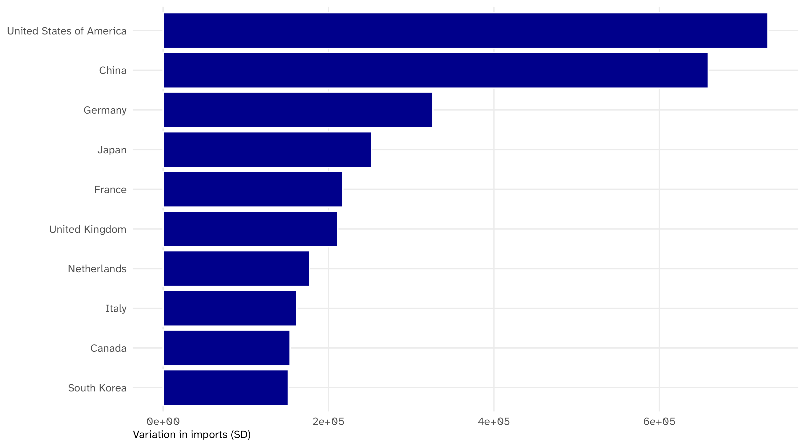
Since the result is a nice, long-format table, we can plot it easily
# A tibble: 10 × 2
  country                  var_trade
  <chr>                        <dbl>
1 United States of America   731302.
2 China                      659178.
3 Germany                    326301.
4 Japan                      252126.
5 France                     217405.
# ℹ 5 more rows
The biggest economies vary the most
Using group_by()
We can group_by() any variable:
Using group_by()
We can even group_by() multiple variables:
# A tibble: 60 × 3
# Groups:   year [12]
   year continent avg_life
  <int> <fct>        <dbl>
1  1952 Africa        39.1
2  1952 Americas      53.3
3  1952 Asia          46.3
4  1952 Europe        64.4
5  1952 Oceania       69.3
# ℹ 55 more rows
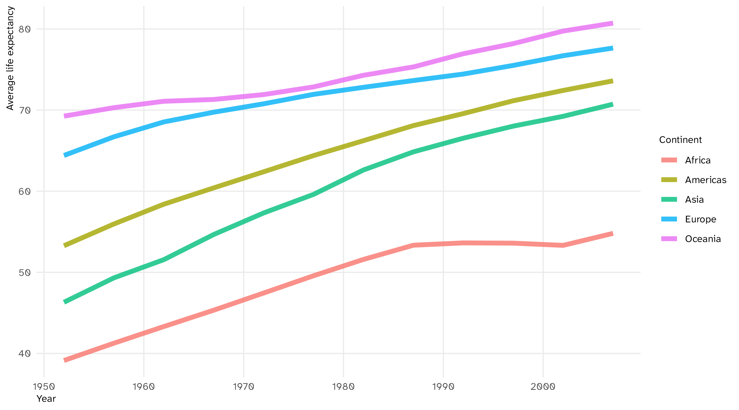
Average life expectancy per continent per year
Using group_by()
Also a nice table we can plot with a grouped time series, since we’re observing each continent over time:
# A tibble: 60 × 3
# Groups:   year [12]
   year continent avg_life
  <int> <fct>        <dbl>
1  1952 Africa        39.1
2  1952 Americas      53.3
3  1952 Asia          46.3
4  1952 Europe        64.4
5  1952 Oceania       69.3
# ℹ 55 more rows
Life expectancy rose everywhere, but Africa stalled after 1990
Report the n behind every average
Which continent had the highest life expectancy in 2007?
# A tibble: 5 × 3
  continent avg_life     n
  <fct>        <dbl> <int>
1 Oceania       80.7     2
2 Europe        77.6    30
3 Americas      73.6    25
4 Asia          70.7    33
5 Africa        54.8    52
Oceania “wins” with two countries. n() counts the rows in each group; put it in every grouped summary so you know what an average is made of
group_by() works with other wrangling functions
Say I wanted to find the top fundraiser in each state in the bonica dataset
I can combine group_by() with slice_max() to do this:
# A tibble: 53 × 4
# Groups:   state [50]
  state name               party total_receipts
  <chr> <chr>              <chr>          <dbl>
1 AK    Galvin, Alyse      I           1479853.
2 AL    Jones, Doug        D          25083352.
3 AR    Hill, James French R           2724802.
4 AZ    Sinema, Kyrsten    D          19287250.
5 AZ    Sinema, Kyrsten    D          19287250.
# ℹ 48 more rows
group_by() works with other wrangling functions
Which county has the highest household income in each state?
Here I can combine group_by() with filter() to do this:
# A tibble: 50 × 3
# Groups:   state [50]
  state name               hh_income
  <chr> <chr>                  <dbl>
1 AL    Shelby County          68770
2 AZ    Maricopa County        53596
3 AR    Saline County          55348
4 CA    Santa Clara County     91702
5 CO    Douglas County        101591
# ℹ 45 more rows
max() is computed within each state, so the filter keeps one county per state
🚨 Your turn: who serves? 🚨
Back to leader:
What share of leaders served in the military, by gender?
Ask your agent: “What share of leaders of each gender have a graduate degree (
edu)? Tell me how you handled missing values.”Now ask it to redo the calculation with the missing leaders kept in the denominator. Did the numbers change? Which version answers the question you asked?
Analyzing categorical data
Analyzing categorical data
Some variables have values that are categories (race, sex, etc.)
Can’t take the mean, median, etc. of a category
But we can look at the proportions of observations in each category, and look for patterns there
Leader education
What level of education do world leaders typically have?
| country | leader | edu |
|---|---|---|
| VEN | Sanabria | Graduate |
| ECU | Paez | Graduate |
| ICE | Hafstein | Graduate |
| IRE | LeMass | Secondary |
| NEP | Juddha Rana | Secondary |
| SAL | Cordova | University |
| FRN | Chirac | Graduate |
| PAK | Sharif | University |
| SEN | Senghor | Graduate |
| GUY | Bharrat Jagdeo | Graduate |
Counting categories
We can use count() to tabulate how many observations are in each category:
# A tibble: 17,686 × 16
  country gwcode leader gender  year yr_office   age edu      mil_service combat
  <chr>    <dbl> <chr>  <chr>  <dbl>     <dbl> <dbl> <fct>          <dbl>  <dbl>
1 USA          2 Grant  M       1869         1    47 Univers…           1      1
2 USA          2 Grant  M       1870         2    48 Univers…           1      1
3 USA          2 Grant  M       1871         3    49 Univers…           1      1
4 USA          2 Grant  M       1872         4    50 Univers…           1      1
5 USA          2 Grant  M       1873         5    51 Univers…           1      1
# ℹ 17,681 more rows
# ℹ 6 more variables: rebel <dbl>, yrs_exp <dbl>, phys_health <dbl>,
#   mental_health <dbl>, will_force <dbl>, will_force_sd <dbl>
Counting categories
We can use count() to tabulate how many observations are in each category:
From counts to percents
We can then use mutate() to calculate the percent in each group:
# A tibble: 5 × 3
  edu            n percent
  <fct>      <int>   <dbl>
1 Primary     1068    6.04
2 Secondary   2856   16.1
3 University  5505   31.1
4 Graduate    5715   32.3
5 <NA>        2542   14.4
\(\text{Primary}_{\%} = \frac{n}{\text{sum}(n)} \times 100 \rightarrow \frac{1068}{(1068 + 2856 + 5505 + 5715 + 2542)} \times 100 = 6.04\%\)
Dealing with NAs
By default, count() will include NA as a category
Cross-tabulations
We can also use count() to do cross-tabulations of two categorical variables
What percent of politicians in bonica are incumbents vs. challengers, by seat type (House vs. Senate)?
# A tibble: 6 × 4
  incumbent  seat       n percent
  <chr>      <chr>  <int>   <dbl>
1 challenger house   6035   61.7
2 challenger senate  1106   11.3
3 incumbent  house   1293   13.2
4 incumbent  senate   108    1.10
5 open seat  house    988   10.1
6 open seat  senate   257    2.63
Incumbents are 1% of Senate candidates? Read the denominator: sum(n) is all 9,787 politicians. That’s the percent of everyone who is a Senate incumbent
Percent of what?
The question was by seat type: within House races, and within Senate races
group_by(seat) before mutate(), and sum(n) is computed within each seat:
# A tibble: 6 × 4
# Groups:   seat [2]
  incumbent  seat       n percent
  <chr>      <chr>  <int>   <dbl>
1 challenger house   6035   72.6
2 challenger senate  1106   75.2
3 incumbent  house   1293   15.5
4 incumbent  senate   108    7.34
5 open seat  house    988   11.9
6 open seat  senate   257   17.5
Now each seat sums to 100. Incumbents are 7% of Senate candidates, not 1%
Rule: say what it’s a percent of
Same six counts, two different answers. What changed is the denominator
Before you report a percent, say the denominator out loud: percent of all politicians, or percent of Senate candidates? group_by() is what decides
The agent will pick a denominator for you. Read the code and check which one
🚨 Your turn: coups 🚨
The coups dataset from juanr has one row per coup event: every known failed and successful attempt, worldwide
| country | year | realized | military | injured | jailed | tried | fled | exile |
|---|---|---|---|---|---|---|---|---|
| Afghanistan | 1963 | 1 | 0 | 0 | 0 | 0 | 0 | 0 |
| Afghanistan | 1973 | 1 | 1 | 0 | 0 | 0 | 1 | 0 |
| Afghanistan | 1973 | 0 | 1 | 0 | 0 | 0 | 0 | 0 |
| Afghanistan | 1976 | 0 | 1 | 0 | 0 | 0 | 0 | 0 |
| Afghanistan | 1978 | 1 | 1 | 0 | 0 | 0 | 0 | 0 |
| Afghanistan | 1979 | 1 | 0 | 0 | 0 | 0 | 0 | 0 |
Your turn: coups
What percent of all known coup attempts succeed (
realized)?What percent of coups end with the leader jailed (
jailed)? Fleeing (fled)? Exiled (exile)? Onesummarize(), three numbersWhat percent of all coup attempts are led by the military (
military) and succeed?Ask your agent: “Are coups more likely to succeed when the military leads them?” Read its code. Is its percent out of all coups, or within military and non-military coups? Only one of those answers the question
This afternoon
Problem set 4
Inside your camp project, write code/04_set.R that answers the questions in the problem set.
It is your script: for any line in it, you should be able to say what it does.
New today: for every summary, say how many rows were missing and whether they are in the denominator. For every percent, say what it is a percent of.
When you think you’re done: restart R and run the script top to bottom. If it works then, it works.